Month: April 2025

  • Understanding TCP/IP: Layers, Protocols, Addressing, and Delivery

    Understanding TCP/IP: Layers, Protocols, Addressing, and Delivery

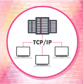
    “Learn TCP/IP in a Weekend” introduces the fundamental TCP/IP model and compares it to the OSI model, emphasizing data encapsulation and fragmentation. It explains the four layers of TCP/IP, their functions, associated protocols like TCP and IP, and concepts such as protocol binding and MTU black holes. The course further covers essential TCP/IP protocols like UDP, ARP, RARP, ICMP, and IGMP, detailing their roles in network communication. Additionally, it explains IP addressing, subnetting, and the distinction between IPv4 and IPv6, including addressing schemes, classes, reserved addresses, and subnet masks. Finally, the material examines common TCP/IP tools and commands for network diagnostics and configuration, along with principles of remote access and security using IPSec.

    Network Fundamentals Study Guide

    Quiz

    1. Explain the process of IP fragmentation. When does it occur, and how does the receiving end handle it? IP fragmentation occurs when a transmitting device sends a datagram larger than the MTU of a network device along the path. The transmitting internet layer divides the datagram into smaller fragments. The receiving end’s internet layer then reassembles these fragments based on information in the header, such as the “more fragments” bit.
    2. Describe what a black hole router is and why it poses a problem for network communication. A black hole router is a router that receives a datagram larger than its MTU and should send an ICMP “destination unreachable” message back, but this message is blocked (often by a firewall). As a result, the sender never receives notification of the problem, and the data is lost without explanation, disappearing as if into a black hole.
    3. What is the purpose of the MAC address, and how is it structured? The MAC (Media Access Control) address is a 48-bit hexadecimal universally unique identifier that serves as the physical address of a network interface card (NIC). It’s structured into two main parts: the first part is the OUI (Organizational Unique Identifier), which identifies the manufacturer, and the second part is specific to that individual device.
    4. Outline the key components of an Ethernet frame and their functions. An Ethernet frame includes the preamble (synchronization), the start of frame delimiter (indicates the beginning of data), the destination MAC address (recipient’s physical address), and the source MAC address (sender’s physical address). These components ensure proper delivery and identification of the data on a local network.
    5. Explain the primary functions of ARP (Address Resolution Protocol) and RARP (Reverse Address Resolution Protocol). ARP is used to resolve an IP address to its corresponding MAC address on a local network, enabling communication between devices. RARP performs the opposite function, mapping a MAC address to its assigned IP address, though it is less commonly used today.
    6. What is the role of ICMP (Internet Control Message Protocol) in networking? Provide an example of its use. ICMP is a protocol used to send messages related to the status of a system and for diagnostic or testing purposes, rather than for sending regular data. An example of its use is the ping utility, which uses ICMP echo requests and replies to determine the connectivity status of a target system.
    7. Differentiate between TCP (Transmission Control Protocol) and UDP (User Datagram Protocol). TCP is a connection-oriented protocol that provides reliable, ordered, and error-checked delivery of data through mechanisms like acknowledgements and retransmissions. UDP is a connectionless protocol that offers faster, less overhead communication but does not guarantee delivery or order.
    8. Describe the three main port ranges defined by the IANA (Internet Assigned Numbers Authority). The three main port ranges are: well-known ports (1-1023), which are assigned to common services; registered ports (1024-49151), which can be registered by applications; and dynamic or private ports (49152-65535), which are used for temporary connections and unregistered services.
    9. Explain the purpose of a subnet mask and how it helps in network segmentation. A subnet mask is a 32-bit binary number that separates the network portion of an IP address from the host portion. By defining which bits belong to the network and which belong to the host, it enables the creation of subnets, which are smaller logical divisions within a larger network, improving organization and efficiency.
    10. What is a default gateway, and why is it necessary for a device to communicate with hosts on different networks? A default gateway is the IP address of a router on the local network that a device sends traffic to when the destination IP address is outside of its own network. It acts as a forwarding point, allowing devices on one network to communicate with devices on other networks by routing traffic appropriately.

    Essay Format Questions

    1. Discuss the evolution from IPv4 to IPv6, highlighting the key limitations of IPv4 that necessitated the development of IPv6 and the primary advantages offered by the newer protocol.
    2. Compare and contrast the TCP/IP model with the OSI model, explaining the layers in each model and how they correspond to one another in terms of network functionality.
    3. Analyze the importance of network security protocols such as IPSec in maintaining data confidentiality, integrity, and availability in modern network environments.
    4. Describe the role of dynamic IP addressing using DHCP in network administration, including the benefits and potential challenges compared to static IP addressing.
    5. Evaluate the significance of various TCP/IP tools and commands (e.g., ping, traceroute, nslookup) in network troubleshooting, diagnostics, and security analysis.

    Glossary of Key Terms

    • Datagram: A basic unit of data transfer in a packet-switched network, particularly in connectionless protocols like IP and UDP.
    • MTU (Maximum Transmission Unit): The largest size (in bytes) of a protocol data unit that can be transmitted in a single network layer transaction.
    • Fragmentation: The process of dividing a large datagram into smaller pieces (fragments) to accommodate the MTU limitations of network devices along the transmission path.
    • Reassembly: The process at the receiving end of reconstructing the original datagram from its fragmented pieces.
    • Flag Bits (DF and MF): Fields within the IP header used during fragmentation. The DF (Don’t Fragment) bit indicates whether fragmentation is allowed, and the MF (More Fragments) bit indicates if there are more fragments to follow.
    • Black Hole Router: A router that drops datagrams that are too large without sending an ICMP “destination unreachable” message back to the source, typically due to a blocked ICMP response.
    • ICMP (Internet Control Message Protocol): A network layer protocol used for error reporting and diagnostic functions, such as the ping utility.
    • Network Interface Layer (TCP/IP): The lowest layer in the TCP/IP model, responsible for the physical transmission of data across the network medium; corresponds to the Physical and Data Link layers of the OSI model.
    • Frame: A data unit at the Data Link layer of the OSI model (and conceptually at the Network Interface Layer of TCP/IP), containing header and trailer information along with the payload (data).
    • MAC Address (Media Access Control Address): A unique 48-bit hexadecimal identifier assigned to a network interface card for communication on a local network.
    • OUI (Organizational Unique Identifier): The first 24 bits of a MAC address, identifying the manufacturer of the network interface.
    • Preamble: A 7-byte (56-bit) sequence at the beginning of an Ethernet frame used for synchronization between the sending and receiving devices.
    • Start of Frame Delimiter (SFD): A 1-byte (8-bit) field in an Ethernet frame that signals the beginning of the actual data transmission.
    • TCP (Transmission Control Protocol): A connection-oriented, reliable transport layer protocol that provides ordered and error-checked delivery of data.
    • IP (Internet Protocol): A network layer protocol responsible for addressing and routing packets across a network.
    • UDP (User Datagram Protocol): A connectionless, unreliable transport layer protocol that offers faster communication with less overhead than TCP.
    • ARP (Address Resolution Protocol): A protocol used to map IP addresses to their corresponding MAC addresses on a local network.
    • RARP (Reverse Address Resolution Protocol): A protocol used (less commonly today) to map MAC addresses to IP addresses.
    • IGMP (Internet Group Management Protocol): A protocol used by hosts and routers to manage membership in multicast groups.
    • Multicast: A method of sending data to a group of interested recipients simultaneously.
    • Unicast: A method of sending data from one sender to a single receiver.
    • Binary: A base-2 number system using only the digits 0 and 1.
    • Decimal: A base-10 number system using the digits 0 through 9.
    • Octet: An 8-bit unit of data, commonly used in IP addressing.
    • Port (Networking): A logical endpoint for communication in computer networking, identifying a specific process or application.
    • IANA (Internet Assigned Numbers Authority): The organization responsible for the global coordination of IP addresses, domain names, and protocol parameters, including port numbers.
    • Well-Known Ports: Port numbers ranging from 0 to 1023, reserved for common network services and protocols.
    • Registered Ports: Port numbers ranging from 1024 to 49151, which can be registered by applications.
    • Dynamic/Private Ports: Port numbers ranging from 49152 to 65535, used for temporary or private connections.
    • FTP (File Transfer Protocol): A standard network protocol used for the transfer of computer files between a client and server on a computer network.
    • NTP (Network Time Protocol): A protocol used to synchronize the clocks of computer systems over a network.
    • SMTP (Simple Mail Transfer Protocol): A protocol used for sending email between mail servers.
    • POP3 (Post Office Protocol version 3): An application layer protocol used by email clients to retrieve email from a mail server.
    • IMAP (Internet Message Access Protocol): An application layer protocol used by email clients to access email on a mail server.
    • NNTP (Network News Transfer Protocol): An application layer protocol used for transporting Usenet news articles.
    • HTTP (Hypertext Transfer Protocol): The foundation of data communication for the World Wide Web.
    • HTTPS (Hypertext Transfer Protocol Secure): A secure version of HTTP that uses encryption (SSL/TLS) for secure communication.
    • RDP (Remote Desktop Protocol): A proprietary protocol developed by Microsoft which provides a user with a graphical interface to connect to another computer over a network connection.
    • DNS (Domain Name System): A hierarchical and decentralized naming system for computers, services, or other resources connected to the Internet or a private network, translating domain names to IP addresses.
    • FQDN (Fully Qualified Domain Name): A complete domain name that uniquely identifies a host on the Internet.
    • WINS (Windows Internet Naming Service): A Microsoft service for NetBIOS name resolution on a network.
    • NetBIOS (Network Basic Input/Output System): A networking protocol that provides services related to the transport and session layers of the OSI model.
    • IPv4 (Internet Protocol version 4): The fourth version of the Internet Protocol, using 32-bit addresses.
    • Octet (in IP addressing): One of the four 8-bit sections of an IPv4 address, typically written in decimal form separated by dots.
    • Subnetting: The practice of dividing a network into smaller subnetworks (subnets) to improve network organization and efficiency.
    • Subnet Mask: A 32-bit number that distinguishes the network portion of an IP address from the host portion, used in IP configuration to define the subnet.
    • Network ID: The portion of an IP address that identifies the network to which the host belongs.
    • Host ID: The portion of an IP address that identifies a specific device (host) within a network.
    • ANDing (Bitwise AND): A logical operation used in subnetting to determine the network address by comparing the IP address and the subnet mask in binary form.
    • Classful IP Addressing: An older system of IP addressing that divided IP addresses into five classes (A, B, C, D, E) with predefined network and host portions.
    • Classless IP Addressing (CIDR – Classless Inter-Domain Routing): A more flexible IP addressing system that allows for variable-length subnet masks (VLSM), indicated by a slash followed by the number of network bits (e.g., /24).
    • Reserved IP Addresses: IP addresses that are not intended for public use and have special purposes (e.g., loopback address 127.0.0.1).
    • Private IP Addresses: Ranges of IP addresses defined for use within private networks, not routable on the public internet (e.g., 192.168.x.x).
    • Public IP Addresses: IP addresses that are routable on the public internet and are typically assigned by an ISP.
    • Loopback Address: An IP address (127.0.0.1 for IPv4, ::1 for IPv6) used for testing the network stack on a local machine.
    • Broadcast Address: An IP address within a network segment that is used to send messages to all devices in that segment (e.g., the last address in a subnet).
    • Default Gateway: The IP address of a router that serves as an access point to other networks, typically the internet.
    • VLSM (Variable Length Subnet Mask): A subnetting technique that allows different subnets within the same network to have different subnet masks, enabling more efficient use of IP addresses.
    • CIDR (Classless Inter-Domain Routing): An IP addressing scheme that replaces the older classful addressing architecture, using VLSM and representing networks by an IP address and a prefix length (e.g., 192.168.1.0/24).
    • Supernetting: The process of combining multiple smaller network segments into a larger network segment, often using CIDR notation with a shorter prefix length.
    • IPv6 (Internet Protocol version 6): The latest version of the Internet Protocol, using 128-bit addresses, intended to address the limitations of IPv4.
    • Hexadecimal: A base-16 number system using the digits 0-9 and the letters A-F.
    • IPv6 Address Format: Consists of eight groups of four hexadecimal digits, separated by colons.
    • IPv6 Address Compression: Rules for shortening IPv6 addresses by omitting leading zeros and replacing consecutive zero groups with a double colon (::).
    • Global Unicast Address (IPv6): A publicly routable IPv6 address, similar to public IPv4 addresses.
    • Unique Local Address (IPv6): An IPv6 address intended for private networks, not globally routable.
    • Link-Local Address (IPv6): An IPv6 address that is only valid within a single network link, often starting with FE80.
    • Multicast Address (IPv6): An IPv6 address that identifies a group of interfaces, used for one-to-many communication.
    • Anycast Address (IPv6): An IPv6 address that identifies a set of interfaces (typically belonging to different nodes), with packets addressed to an anycast address being routed to the nearest interface in the set.
    • EUI-64 (Extended Unique Identifier-64): A method for automatically configuring IPv6 interface IDs based on the 48-bit MAC address, with a 64-bit format.
    • Neighbor Discovery Protocol (NDP): A protocol used by IPv6 nodes to discover other nodes on the same link, determine their link-layer addresses, find available routers, and perform address autoconfiguration.
    • Router Solicitation (RS): An NDP message sent by a host to request routers to send router advertisements immediately.
    • Router Advertisement (RA): An NDP message sent by routers to advertise their presence, link parameters, and IPv6 prefixes.
    • Neighbor Solicitation (NS): An NDP message sent by a node to determine the link-layer address of a neighbor or to verify that a neighbor is still reachable.
    • Neighbor Advertisement (NA): An NDP message sent by a node in response to a neighbor solicitation or to announce a change in its link-layer address.
    • DAD (Duplicate Address Detection): A process in IPv6 used to ensure that a newly configured unicast address is unique on the link.
    • DHCPv6 (Dynamic Host Configuration Protocol for IPv6): A network protocol used by IPv6 hosts to obtain configuration information such as IPv6 addresses, DNS server addresses, and other configuration parameters from a DHCPv6 server.
    • Tunneling (Networking): A technique that allows network packets to be encapsulated within packets of another protocol, often used to transmit IPv6 traffic over an IPv4 network.
    • ISATAP (Intra-Site Automatic Tunnel Addressing Protocol): An IPv6 transition mechanism that allows IPv6 hosts to communicate over an IPv4 network by encapsulating IPv6 packets within IPv4 packets.
    • 6to4: An IPv6 transition mechanism that allows IPv6 networks to communicate over the IPv4 Internet without explicit configuration of tunnels.
    • Teredo: An IPv6 transition mechanism that provides IPv6 connectivity to IPv6-aware hosts that are located behind NAT devices and have only IPv4 connectivity to the Internet.
    • Netstat: A command-line utility that displays network connections, listening ports, Ethernet statistics, the IP routing table, IPv4 statistics (for IP, ICMP, TCP, and UDP protocols), IPv6 statistics (for IPv6, ICMPv6, TCP over IPv6, and UDP over IPv6), and network interface statistics.
    • Nbtstat: A command-line utility used to diagnose NetBIOS name resolution problems.
    • Nslookup: A command-line tool used to query the Domain Name System (DNS) to obtain domain name or IP address mapping information.
    • Dig (Domain Information Groper): A network command-line tool used to query DNS name servers.
    • Ping: A network utility used to test the reachability of a host on an Internet Protocol (IP) network by sending ICMP echo request packets to the target host and listening for ICMP echo reply packets in return.
    • Traceroute (or Tracert on Windows): A network diagnostic tool for displaying the route (path) and measuring transit delays of packets across an Internet Protocol (IP) network.
    • Protocol Analyzer (Network Analyzer/Packet Sniffer): A tool used to capture and analyze network traffic, allowing inspection of the contents of individual packets.
    • Port Scanner: A program used to probe a server or host for open ports, often used for security assessments or by attackers to find potential entry points.
    • ARP Command: A command-line utility used to view and modify the Address Resolution Protocol (ARP) cache of a computer.
    • Route Command: A command-line utility used to display and manipulate the IP routing table of a computer.
    • DHCP (Dynamic Host Configuration Protocol): A network protocol that enables a server to automatically assign IP addresses and other network configuration parameters to devices on a network.
    • DHCP Scope: The range of IP addresses that a DHCP server is configured to lease to clients on a network.
    • DHCP Lease: The duration of time for which a DHCP client is allowed to use an IP address assigned by a DHCP server.
    • Static IP Addressing: Manually configuring an IP address and other network settings on a device, which remains constant unless manually changed.
    • Dynamic IP Addressing: Obtaining an IP address and other network settings automatically from a DHCP server.
    • APIPA (Automatic Private IP Addressing): A feature in Windows that automatically assigns an IP address in the 169.254.x.x range to a client when a DHCP server is unavailable.
    • VPN (Virtual Private Network): A network that uses a public telecommunications infrastructure, such as the internet, to provide remote offices or individual users with secure access to their organization’s network.
    • Tunneling (in VPNs): The process of encapsulating data packets within other packets to create a secure connection (tunnel) across a public network.
    • RADIUS (Remote Authentication Dial-In User Service): A networking protocol that provides centralized Authentication, Authorization, and Accounting (AAA) management for users who connect to and use a network service.
    • TACACS+ (Terminal Access Controller Access-Control System Plus): A Cisco-proprietary protocol that provides centralized authentication, authorization, and accounting (AAA) for network access.
    • Diameter: An authentication, authorization, and accounting protocol that is intended to overcome some of the limitations of RADIUS.
    • AAA (Authentication, Authorization, Accounting): A security framework that controls who is permitted to use a network (authentication), what they can do once they are on the network (authorization), and keeps a record of their activity (accounting).
    • IPSec (IP Security): A suite of protocols used to secure Internet Protocol (IP) communications by authenticating and/or encrypting each IP packet of a communication session.
    • AH (Authentication Header): An IPSec protocol that provides data origin authentication, data integrity, and anti-replay protection.
    • ESP (Encapsulating Security Payload): An IPSec protocol that provides confidentiality (encryption), data origin authentication, data integrity, and anti-replay protection.
    • Security Association (SA): A simplex (one-way) connection established between a sender and a receiver that provides security services. IPSec peers establish SAs for secure communication.
    • IKE (Internet Key Exchange): A protocol used to establish security associations (SAs) in IPSec.
    • IPSec Policy: A set of rules that define how IPSec should be applied to network traffic, including which traffic should be protected and what security services should be used.

    Briefing Document: Network Fundamentals and Security

    Date: October 26, 2023 Prepared For: [Intended Audience – e.g., Network Engineering Team, Security Analysts] Prepared By: Gemini AI Subject: Review of Network Fundamentals, Addressing, Protocols, Tools, and Security Concepts from Provided Sources

    This briefing document summarizes the key themes, important ideas, and facts discussed in the provided excerpts, covering fundamental networking concepts, IP addressing (both IPv4 and IPv6), essential networking protocols and tools, remote access methods, and security principles.

    Main Themes and Important Ideas

    1. Data Transmission and Fragmentation (01.pdf)

    • When network devices encounter datagrams larger than their Maximum Transmission Unit (MTU), the transmitting internet layer fragments the data into smaller blocks for easier transit.
    • “In these instances when there is a datagramgram that’s larger than the MTU of a device the transmitting internet layer fragments the data or the datagramgram and then tries to resend it in smaller and more easily manageable blocks.”
    • The header of fragmented datagrams contains flag bits: a reserved bit (always zero), the “Don’t Fragment” (DF) bit (on or off), and the “More Fragments” (MF) bit (on if more fragments are coming, off otherwise).
    • “The second is the don’t fragment or the DF bit Now either this bit is off or zero which means fragment this datagram or on meaning don’t fragment this datagram The third flag bit is the more fragments bit MF And when this is on it means that there are more fragments on the way And finally when the MF flag is off it means there are no more fragments to be sent as you can see right here And that there were never any fragments to send.”
    • A “black hole router” occurs when a datagram with an MTU larger than a receiving device’s MTU is sent, and the expected ICMP response notifying the sender of the mismatch is blocked (e.g., by a firewall), leading to data loss.
    • “Now a black hole router is the name given to a situation where a datagramgram is sent with an MTU that’s greater than the MTU of the receiving device as we can see here. Now when the destination device is unable to receive the IP datagramgram it’s supposed to send a specific ICMP response that notifies the transmitting station that there’s an MTU mismatch. This can be due to a variety of reasons one of which could be as simple as a firewall that’s blocking the MP response. … In these cases this is called a black hole because of the disappearance of datagramgrams…”
    • The ping utility can be used to detect MTU black holes by specifying the MTU size in the ICMP echo request.
    • “And one of the best ways is to use the ping utility and specify a syntax that sets the MTU of the ICMP echo request meaning you tell it I want to ping with this much of an MTU And so then we can see if the ping’s not coming back if it’s coming back at one MTU and not another then we know oh this is what’s happening right here.”

    2. Network Interface Layer and Ethernet Frames (01.pdf)

    • The network interface layer (bottom of TCP/IP stack) handles the physical transfer of bits across the network medium and corresponds to the physical and data link layers of the OSI model.
    • Data at this layer is referred to as “frames,” and major functions include layer 2 switching operations based on MAC addresses.
    • A MAC (Media Access Control) address is a 48-bit hexadecimal universally unique identifier, composed of the Organizational Unique Identifier (OUI) and a device-specific part.
    • “A MAC address again is a 48 bit hexadesimal universally unique identifier that’s broken up into several parts The first part of it is what we call the OUI or the organizational unique identifier This basically says what company is uh sending out this device And then we have the second part which is the nick specific…”
    • The structure of an Ethernet frame includes:
    • Preamble (7 bytes/56 bits): Synchronization.
    • Start of Frame Delimiter: Indicates the start of data.
    • Source and Destination MAC Addresses (12 bytes/96 bits total).
    • “The preamble of an Ethernet frame is made up of seven bytes or 56 bits And this serves as synchronization and gives the receiving station a heads up to standby and look out for a signal that’s coming The next part is what we call the start of frame delimiter The only purpose of this is to indicate the start of data The next two parts are the source and destination MAC addresses…”

    3. TCP/IP Protocol Suite and Core Protocols (01.pdf)

    • The TCP/IP protocol suite includes essential protocols like TCP (connection-oriented, reliable), IP (connectionless, routing), UDP (connectionless, fast), ARP (IP to MAC address mapping), RARP (MAC to IP address mapping), ICMP (status and error messages), and IGMP (multicast group management).
    • ARP resolves IP addresses to MAC addresses for local network communication. If the MAC address isn’t in the ARP cache, a broadcast is sent. The target device responds with a unicast containing its MAC address, which is then added to the ARP table.
    • “The ARP process works by first uh receiving the IP address from IP or the internet protocol Then ARP has the MAC address in its cached table So the router has what are called ARP tables that link IP addresses to MAC addresses We call this the ARP table It looks in there to see if it know if it has a MAC address for the IP address listed It then sends it back to the IP if it uh if it does have it And if it doesn’t have it it broadcasts the message it’s sent in order to resolve what we call resolve the address to a MAC address And the target computer with the IP address responds to that broadcast message with what’s called a uniccast message… that contains the MAC address that it’s seeking ARP then will add the MAC address to its table.”
    • ICMP (Internet Control Message Protocol) is used for diagnostic and testing purposes (e.g., ping, traceroute) and to report errors (e.g., MTU black hole notification). It operates at the internet layer.
    • “ICMP which is also called the internet control message protocol It’s a protocol designed to send messages that relate to the status of a system It’s not meant to actually send data So ICMP messages are used generally speaking for diagnostic and testing purposes Now they can also be used as a response to errors that occur in the normal operations of IP And if you recall one of the times that we talked about that was for instance with the MTU black hole when that MP message couldn’t get back to the original router.”
    • IGMP (Internet Group Management Protocol) manages membership in multicast groups, allowing one-to-many communication.

    4. IP Packet Delivery and Binary/Decimal Conversion (01.pdf)

    • IP packet delivery involves resolving the host name to an IP address (using services like DNS), establishing a connection at the transport layer, determining if the destination is local or remote based on the subnet mask, and then routing and delivering the packet.
    • Understanding binary (base 2) and decimal (base 10) conversions is crucial for IP addressing and subnetting. Binary uses 0s and 1s, while decimal uses 0-9. An octet is an 8-bit binary number.
    • Conversion between binary and decimal involves understanding the place values (powers of 2 for binary, powers of 10 for decimal).

    5. Network Ports and Protocols (01.pdf)

    • A network port is a process-specific or application-specific designation that serves as a communication endpoint in a computer’s operating system.
    • The Internet Assigned Numbers Authority (IANA) regulates port assignments, which range from 0 to over 65,000 (port 0 is reserved).
    • Port ranges are divided into three subsets:
    • Well-known ports (1-1023): Used by common services.
    • Registered ports (1024-49151): Reserved by applications that register with IANA.
    • Dynamic/private ports (49152-65535): Used by unregistered services and for temporary connections.
    • Key well-known ports and their associated protocols include:
    • 7: Echo (used by ping).
    • 20, 21: FTP (File Transfer Protocol) – data and control.
    • 22: SSH (Secure Shell).
    • 23: Telnet.
    • 25: SMTP (Simple Mail Transfer Protocol) – sending email.
    • 53: DNS (Domain Name Service).
    • 67, 68: DHCP (Dynamic Host Configuration Protocol) and BOOTP.
    • 69: TFTP (Trivial File Transfer Protocol).
    • 80: HTTP (Hypertext Transfer Protocol).
    • 110: POP3 (Post Office Protocol version 3) – receiving email.
    • 143: IMAP (Internet Message Access Protocol) – accessing email.
    • 443: HTTPS (HTTP Secure).
    • 3389: RDP (Remote Desktop Protocol).
    • 123: NTP (Network Time Protocol).
    • 119: NNTP (Network News Transfer Protocol).

    6. Network Addressing: Names, Addresses, and IPv4 (01.pdf)

    • Devices communicate using network addresses (IP addresses). Naming services map network names (e.g., hostnames, domain names) to these addresses.
    • Common network naming services:
    • DNS (Domain Name Service): Used on the internet and most networks to translate fully qualified domain names (FQDNs) to IP addresses.
    • WINS (Windows Internet Naming Service): Outdated Windows-specific service.
    • NetBIOS: Broadcast-based service used on Windows networks.
    • IPv4 addresses are 32-bit binary addresses, typically represented in dotted decimal format (four octets).
    • “IPv4 IP version 4 addresses is a very important aspect of networking for any administrator or uh technician or even just uh you know IT guy to understand It is a 32bit binary address that’s used to identify and differentiate nodes on a network In other words it is your address on the network or your social security number with the IPv4 addressing scheme being a 32bit address And you can see if we counted each one of these up remember a bit is either zero or one And we can count up there are 32 of these.”
    • Theoretically, IPv4 allows for approximately 4.29 billion unique addresses.
    • IP addresses are managed by IANA (Internet Assigned Numbers Authority) and Regional Internet Registries (RIRs).

    7. Subnetting and Subnet Masks (01.pdf)

    • Subnetting divides a larger network into smaller subnetworks to improve routing efficiency, management, and security.
    • A subnet mask is a 32-bit binary address (similar to an IP address) used to separate the network portion from the node portion of an IP address.
    • “A subnet mask is like an IP address a 32bit binary address broken up into four octets in a dotted decimal format just like an IP address And it’s used to separate the network portion from the node portion I’m going to show you how that works in just a minute.”
    • Applying a subnet mask to an IP address using a bitwise AND operation reveals the network ID.
    • “When a subnet mask is applied to an IP address the remainder is the network portion Meaning when we take the IP address and we apply the subnet mask and I’ll show you how to do that in a second what we get as a remainder what’s left over is going to be the network ID This allows us to then determine what the node ID is This will make more sense in just a minute The way we do this is through something called ending Anding is a mathematics term It really has to do with logic The way it works is and you just have to sort of remember these rules One and one is one One and zero is zero And the trick there is that that zero is there 0 and 1 is zero And 0 and 0 is also zero So basically what ending does is allows us to hide certain um address certain bits from the rest of the network and therefore we’re allowed to get uh the IP address uh or rather the network address from the node address.”
    • Rules for subnet masks: Ones are always contiguous from the left, and zeros are always contiguous from the right.
    • Default subnet masks correspond to IP address classes.
    • Custom subnet masks allow for further division of networks by “borrowing” bits from the host portion for the network portion.

    8. Default and Custom IP Addressing (01.pdf)

    • The default IPv4 addressing scheme is divided into classes (A, B, C, D, E) based on the first octet, determining the number of available networks and hosts.
    • Class A (1-127): Large networks, many hosts. Default subnet mask: 255.0.0.0.
    • Class B (128-191): Mid-sized networks, moderate hosts. Default subnet mask: 255.255.0.0.
    • Class C (192-223): Small networks, fewer hosts. Default subnet mask: 255.255.255.0.
    • Class D (224-239): Multicast.
    • Class E (240-255): Experimental.
    • “As we learned in previous modules the IPv4 addressing scheme is again 32 bits broken up into four octets and each octet can range from 0 to 255 Now the international standards organization I can which we’ve mentioned in a previous module is in control of how these IP addresses are leased and distributed out to individuals and companies around the world Now because of the limited amount of IP addresses the default IPv4 addressing scheme is designed and outlined which what are called classes and there are five of them that we need to know Now these classes are identified as A B C D and E And each class is designed to facilitate in the distribution of IP addresses for certain types of purposes.”
    • Reserved and restricted IPv4 addresses:
    • 127.0.0.1: Loopback address (localhost).
    • Addresses with all zeros or all ones in the host portion (e.g., 0.0.0.0, 255.255.255.255) are typically not assignable (network address and broadcast address, respectively).
    • 1.1.1.1: All hosts or “who is” address (generally unusable).
    • Private IPv4 address ranges (not routable on the public internet):
    • Class A: 10.0.0.0 – 10.255.255.255.
    • Class B: 172.16.0.0 – 172.31.255.255.
    • Class C: 192.168.0.0 – 192.168.255.255.
    • “Private IP addresses are not routable This means that they are assigned for use on internal networks such as your home network or your office network When these addresses transmit data and it reaches a router the router is not going to uh route it outside of the network So these addresses can be used without needing to purchase or leasing an IP address from your ISP or internet service provider or governing entity.”
    • IPv4 Formulas:
    • Number of usable hosts per subnet: 2^x – 2 (where x is the number of host bits).
    • Number of available subnets: 2^y – 2 (where y is the number of network bits borrowed).
    • Default Gateway: The IP address of the router that a local device uses to communicate with networks outside its own subnet (often the internet).
    • “The for any device that wants to connect to the internet has to go through what’s called a default gateway This is not a physical device This is set uh by our IP address settings It is basically the IP address of the device which is usually the router or the border router that’s connected directly to the to the internet.”
    • Custom IP address schemes:
    • VLSM (Variable Length Subnet Mask): Assigns each subnet its own customized subnet mask of varying length, allowing for more efficient IP address allocation.
    • CIDR (Classless Inter-Domain Routing) / Supernetting / Classless Routing: Uses VLSM principles and represents networks using an IP address followed by a slash and a number indicating the number of network bits (e.g., 192.168.13.0/23). This notation simplifies subnetting and has led to classless address space on the internet.

    9. Data Delivery Techniques and IPv6 (01.pdf)

    • IPv6 is the successor to IPv4, offering a significantly larger address space (128-bit addresses).
    • “The first major improvement that came with this new version is that there’s been an exponential increase in the number of possible addresses that are available Uh several other features were added to this addressing scheme as well such as security uh improved composition for what are called uniccast addresses uh header simplification and how they’re sent and uh hierarchal addressing for what some would suggest is easier routing And there’s also a support for what we call time sensitive traffic or traffic that needs to be received in a certain amount of time such as voice over IP and gaming And we’re going to look at all of this shortly. The IPv6 addressing scheme uses a 128 bit binary address This is different of course from IP version 4 which again uses a 32bit address So this means therefore that there are two to 128 power possible uh addresses as opposed to 2 to the 32 power with um IP address 4 And this means therefore that there are around 340 unicilian… addresses.”
    • IPv6 addresses are written in hexadecimal format, with eight groups of four hexadecimal digits separated by colons.
    • IPv6 address shortening rules (truncation):
    • Leading zeros within a group can be omitted.
    • One or more consecutive groups of zeros can be replaced with a double colon (::). This can only be done once in an address.
    • IPv6 has a subnet size of /64 (the first 64 bits represent the network/subnet, the last 64 bits represent the host ID).
    • Data delivery techniques involve connection-oriented (e.g., TCP, reliable, acknowledgment) and connectionless (e.g., UDP, faster, no guarantee) modes.
    • Transmit types include unicast (one-to-one), multicast (one-to-many to interested hosts), and in IPv6, anycast (one-to-nearest of a group). Broadcast, present in IPv4, is not used in IPv6; multicast addresses fulfill similar functions.
    • Data flow control mechanisms:
    • Buffering: Temporary storage of data to manage rate mismatches and ensure consistency. Squelch signals can be sent if buffers are full.
    • Data Windows: Amount of data sent before acknowledgment is required. Can be fixed length or sliding windows (adjusting size based on network conditions). Sliding windows help minimize congestion and maximize throughput.
    • Error detection methods ensure data integrity during transmission (e.g., checksums).

    10. IPv6 Address Types and Features (01.pdf)

    • Main IPv6 address types:
    • Global Unicast: Publicly routable addresses assigned by ISPs (range 2000::/3).
    • Unique Local: Private addresses for internal networks (similar to IPv4 private addresses, deprecated FC00::/7).
    • Link-Local: Non-routable addresses for communication within a single network link (FE80::/10). Automatically configured when IPv6 is enabled. Used for routing protocol communication and neighbor discovery.
    • Multicast: One-to-many communication (FF00::/8). Replaces broadcast in IPv4. Used for duplicate address detection and neighbor discovery.
    • Anycast: One-to-nearest of a group of interfaces (not explicitly detailed but mentioned).
    • IPv6 features:
    • Increased address space.
    • Improved security features (IPSec integration).
    • Simplified header format.
    • Hierarchical addressing for efficient routing.
    • Support for time-sensitive traffic (QoS).
    • Plug-and-play capabilities with mobile devices.
    • Stateless autoconfiguration (SLAAC).
    • EUI-64 Addressing: A method for automatically generating the host portion of an IPv6 address using the 48-bit MAC address of the interface. This involves:
    1. Taking the 48-bit MAC address.
    2. Inserting FFFE in the middle (after the first 24 bits).
    3. Inverting the seventh bit (universal/local bit) of the first octet.
    • Neighbor Discovery Protocol (NDP): Replaces ARP in IPv4. Used for:
    • Router Solicitation (RS): Hosts ask for routers on the link.
    • Router Advertisement (RA): Routers announce their presence and network prefixes.
    • Neighbor Solicitation (NS): Hosts ask for the MAC address (link-layer address) of a neighbor or for duplicate address detection.
    • Neighbor Advertisement (NA): Neighbors reply to NS messages or announce address changes.
    • Duplicate Address Detection (DAD): Ensures IPv6 addresses are unique on the link using Neighbor Solicitation and Advertisement with multicast.
    • DHCPv6: Used for stateful autoconfiguration, allocating IPv6 addresses, DNS server information, and other configuration parameters to hosts. Uses UDP ports 546 (client) and 547 (server).
    • IPv6 Transition Mechanisms: Techniques to allow IPv6 hosts to communicate with IPv4 networks during the transition period, often involving tunneling IPv6 packets within IPv4 headers (e.g., ISATAP).

    11. Static vs. Dynamic IP Addressing and DHCP (01.pdf)

    • Static IP Addressing: Manually assigned IP address that does not change. Requires manual configuration of IP address, subnet mask, and default gateway on each device.
    • Dynamic IP Addressing (DHCP): IP address is automatically assigned by a DHCP server and can change over time.
    • “This is the protocol which assigns IP addresses And it does this first by assigning what’s called or defining rather what’s called the scope The scope are the ranges of all of the available IP address on the system that’s running the DHCP service And what this does is it takes one of the IP addresses from this scope and assigns it to a computer or a client.”
    • DHCP Scope: The range of IP addresses available for assignment by the DHCP server. Exclusions can be configured for static IP addresses.
    • DHCP Lease: The duration for which an IP address is assigned to a client. Clients must renew their lease periodically.
    • Strengths and weaknesses:
    • Static: Reliable for servers and devices needing consistent addresses, but requires more manual configuration and can lead to address conflicts if not managed carefully.
    • Dynamic: Easier to manage for a large number of clients, reduces configuration overhead and potential for conflicts (if DHCP is properly configured), but IP addresses can change.
    • APIPA (Automatic Private IP Addressing): A feature in Windows that automatically assigns an IP address in the 169.254.x.x range to a client if it cannot obtain an IP address from a DHCP server.

    12. TCP/IP Tools and Commands (01.pdf)

    • Essential TCP/IP tools for troubleshooting and network analysis:
    • ping: Sends ICMP echo request packets to test connectivity to a destination host. Measures round-trip time (RTT) and packet loss.
    • “The ping tool and the ping command are extremely useful when it comes to troubleshooting and testing connectivity Basically what the tool does is send a packet of information and that packet again is MP through a connection and waits to see if it receives some packets back.”
    • traceroute (or tracert on Windows): Traces the path that packets take to a destination, showing the sequence of routers (hops) and the RTT at each hop. Uses ICMP time-exceeded messages.
    • “It basically tells us the time it takes for a packet to travel between different routers and devices And we call this the amount of hops along the uh the network So it not only tests where connectivity might have been lost but it’s also going to test um the time that it takes to get from one end to the other end of the connection And it’s also going to also show us the number of hops between those computers.”
    • Protocol Analyzer (Network Analyzer): Captures and analyzes network traffic (packets) in real-time or from a capture file. Provides detailed information about protocols, source/destination addresses, data content, etc. (e.g., Wireshark).
    • “This is an essential tool when you’re running a network It basically gives you a readable report of virtually everything that’s being sent and transferred over your network So these analyzers will capture packets that are going through the network and put them into a buffer zone.”
    • Port Scanner: Scans a network host for open TCP or UDP ports. Used for security assessments (identifying running services) or by attackers to find potential vulnerabilities (e.g., Nmap).
    • “A port scanner does exactly what it sounds like It basically scans the network for open ports either for malicious or for safety reasons So uh it’s usually used by administrators to check the security of their system and make sure nothing’s left open Oppositely it can be used by attackers for their advantage.”
    • nslookup: Queries DNS servers to obtain IP address information for a given domain name or vice versa. Useful for troubleshooting DNS-related issues. dig is a more advanced alternative on Unix/Linux systems.
    • “It’s used to basically find out uh what the server and address information is for a domain that’s queried It’s mostly used to troubleshoot domain name service related items and you can also get information about a systems configuration.”
    • arp: Displays and modifies the ARP cache, which maps IP addresses to MAC addresses on the local network.
    • “It’s really used to find the media access control or MAC address or the physical address for an IP address or vice versa Remember this is the physical address It’s hardwired onto the device The MAC address is the system’s physical address and the IP address is the one again assigned by a server or manually assigned.”
    • route: Displays and modifies the routing table of a host or router, showing the paths that network traffic will take. More commonly used on routers.
    • “Finally the route command is extremely handy and can be used uh fairly often And it basically this shows you the routing table uh which is going to give you a list of all the routing entries.”
    • ipconfig (Windows) / ifconfig (Linux/macOS): Displays and configures network interface parameters, including IP address, subnet mask, default gateway, and DNS server information.

    13. Remote Networking and Access (01.pdf)

    • Remote access allows users to connect to and use network resources from a distance.
    • Key terms and concepts:
    • VPN (Virtual Private Network): Extends a LAN across a wide area network (like the internet) by creating secure, encrypted tunnels. Provides confidentiality and integrity for remote connections.
    • “In essence it extends a LAN or a local area network by adding the ability to have remote users connect to it The way it does this is by using what’s called tunneling It basically creates a tunnel in uh through the wide area network the internet that then I can connect to and through So all of my data is traveling through this tunnel between the server or the corporate office and the client computer This way I can make sure that no one outside the tunnel or anyone else on the network can get in and I can be sure that all of my data is kept secure This is why it’s called a virtual private network It’s virtual It’s not real It’s not physical It’s definitely private because the tunnel makes sure to keep everything out.”
    • RADIUS (Remote Authentication Dial-In User Service): A centralized protocol for authentication, authorization, and accounting (AAA) of users connecting to a network remotely (e.g., VPN access).
    • “What this does is it allows us to have centralized authorization authentication and accounting management for computers and users on a remote network In other words it allows me to have one server that’s going to be responsible and we’re going to call this the Radius server that’s responsible for making sure once a VPN is established that the person on the other end is actually someone who should be connecting to my network.”
    • TACACS+ (Terminal Access Controller Access-Control System Plus): A Cisco-proprietary alternative to RADIUS that also provides centralized AAA services, offering more flexibility in protocol support and separating authorization and authentication.
    • Diameter: Another AAA protocol, initially intended as a more robust replacement for RADIUS.
    • Authentication: Verifying the identity of a user or device.
    • Authorization: Determining what resources or actions an authenticated user is allowed to access or perform.
    • Accounting: Tracking user activity and resource consumption.

    14. IPSec and Security Policies (01.pdf)

    • IPSec (IP Security): A suite of protocols and policies used to secure IP communications by providing confidentiality, integrity, and authentication at the IP layer.
    • “They’re used to provide a secure channel of communication between two systems or more systems These systems can be within a local network within a wide area network or even across the internet.”
    • Key protocols within IPSec:
    • AH (Authentication Header): Provides data integrity and authentication of the sender but does not encrypt the data itself.
    • ESP (Encapsulating Security Payload): Provides data confidentiality (encryption), integrity, and authentication. More commonly used than AH.
    • Services provided by IPSec:
    • Data verification (authentication).
    • Protection from data tampering (integrity).
    • Private transactions (confidentiality through encryption with ESP).
    • IPSec Policies: Define how IPSec is implemented, including the protocols to be used, security algorithms, and key management. These policies are agreed upon by the communicating peers.
    • “IPSec policies dictate the level of security that’s going to be applied to the communication between two or more hosts. These policies need to be configured on each of the systems that are going to be participating in the secure communication and they must agree upon the specific security parameters.”
    • Security principles:
    • CIA Triad (Confidentiality, Integrity, Availability): A fundamental model for information security. IPSec aims to enhance confidentiality and integrity while supporting availability by enabling secure communication channels.

    Conclusion

    The provided sources offer a comprehensive overview of essential networking concepts, ranging from fundamental data transmission mechanisms and addressing schemes (IPv4 and IPv6) to critical protocols, diagnostic tools, remote access technologies, and security principles like IPSec. Understanding these topics is crucial for anyone involved in network administration, security, or IT support. The emphasis on binary/decimal conversion, subnetting, IP address classes, well-known ports, and the functionality of key TCP/IP tools highlights their importance in network operations and troubleshooting. The introduction to IPv6, remote access methods (VPN, RADIUS), and IPSec provides a foundation for understanding modern network security and connectivity solutions.

    Networking Concepts: Answering Frequently Asked Questions

    Frequently Asked Questions about Networking Concepts

    1. What happens when a datagram’s size exceeds the Maximum Transmission Unit (MTU) of a network device?

    When a datagram is larger than a device’s MTU, the transmitting internet layer fragments the datagram into smaller, more manageable blocks. These fragments are then sent, and the receiving end’s internet layer reassembles them back into the original datagram during the reassembly process. The header of these fragmented datagrams includes flag bits: a reserved bit (always zero), the Don’t Fragment (DF) bit (on or off), and the More Fragments (MF) bit (on if more fragments are coming, off if it’s the last or only fragment).

    2. What is an MTU black hole and how can it be detected?

    An MTU black hole occurs when a datagram with an MTU greater than a receiving device’s MTU is sent. The receiving device should send an ICMP response indicating the MTU mismatch, but if this response is blocked (e.g., by a firewall), the sender doesn’t know the datagram was too large, and the data seems to disappear, hence the term “black hole.” One way to detect this is by using the ping utility with a specific syntax to set the MTU of the ICMP echo request. If pings at a certain MTU fail while those at a smaller MTU succeed, it indicates an MTU black hole.

    3. How does the Network Interface Layer (Layer 1 of TCP/IP) function and what data type does it handle?

    The Network Interface Layer is dedicated to the physical transfer of bits across the network medium. It corresponds to the Physical and Data Link Layers of the OSI model. The primary data type handled at this layer is called a “frame.” Major functions include switching operations (at the Data Link/Layer 2 level) that utilize MAC addresses for communication within a local network.

    4. Explain the purpose and components of an Ethernet frame.

    An Ethernet frame is the structure for transmitting data over an Ethernet network. It consists of several parts: * Preamble (7 bytes/56 bits): For synchronization and alerting the receiver. * Start of Frame Delimiter: Indicates the beginning of data. * Destination MAC Address (6 bytes/48 bits): The physical address of the intended recipient. * Source MAC Address (6 bytes/48 bits): The physical address of the sender. These components ensure that data is properly framed, addressed, and synchronized for transmission across the network.

    5. Describe the Address Resolution Protocol (ARP) and its function in network communication.

    ARP is a protocol used to map IP addresses to MAC addresses within a local area network. When a device wants to communicate with another device on the same network using its IP address, ARP is used to find the corresponding MAC address. The sending device broadcasts an ARP request containing the target IP address. The device with that IP address responds with an ARP reply containing its MAC address, allowing direct Layer 2 communication. Routers maintain ARP tables to cache these IP-to-MAC address mappings. RARP (Reverse ARP) performs the opposite function, mapping MAC addresses to IP addresses, though it is less commonly used today.

    6. What are well-known, registered, and dynamic/private port ranges, and why are they important?

    Network ports are logical endpoints for communication in a computer’s operating system, identified by numbers. The Internet Assigned Numbers Authority (IANA) regulates these assignments. The three ranges are: * Well-known ports (1-1023): Used by common services (e.g., HTTP on port 80, SMTP on port 25). Knowing these is crucial for network administration. * Registered ports (1024-49151): Reserved for applications that register with IANA. * Dynamic or private ports (49152-65535): Used for unregistered services, testing, and temporary connections. Understanding these ranges helps in network management, firewall configuration, and troubleshooting.

    7. What are the key differences between IPv4 and IPv6 addressing schemes?

    IPv6 is the successor to IPv4 and offers several improvements. IPv4 uses a 32-bit binary address, allowing for approximately 4.29 billion unique addresses. IPv6 uses a 128-bit binary address, providing a vastly larger address space (around 340 undecillion addresses). IPv6 also features improved security, simplified header format, hierarchical addressing for potentially easier routing, and support for time-sensitive traffic. Unlike IPv4, IPv6 has integrated subnetting (with a standard /64 subnet size) and does not rely on NAT as heavily due to the abundance of addresses. IPv6 addresses are written in hexadecimal format, separated by colons, and can be truncated using specific rules for readability.

    8. Explain the concept of a default gateway and its role in network communication.

    A default gateway is the IP address of a device (usually a router) on a local network that serves as an access point to other networks, including the internet. When a device on the local network needs to communicate with a device outside its own subnet, it sends the traffic to its configured default gateway. The default gateway then routes the traffic towards the destination network. For a device to connect to the internet, it typically needs to be configured with an IP address, a subnet mask, and the IP address of the default gateway.

    TCP/IP Model: Core Concepts of Network Communication

    The TCP/IP model is a widely used networking model that allows for the conceptualization of how a computer network functions in maintaining hardware and protocol interoperability. It is also commonly called the DoD model because much of the research was funded by the Department of Defense. The TCP/IP model was permanently activated in 1983 and commercially marketed starting in 1985. It is now the preferred network standard for protocols. Understanding this model and how data flows within it is essential for all computers using the internet or most networks.

    Key aspects of the TCP/IP model discussed in the sources include:

    • Abstract Layers: Similar to the OSI model, the TCP/IP model is defined using abstract layers. However, the TCP/IP model consists of four layers:
    • Network Interface Layer (Layer 1): This is the bottom layer and is dedicated to the actual transfer of bits across the network medium. It directly correlates to the physical and data link layers of the OSI model. The data type at this layer is called frames. Major functions include switching operations using MAC addresses. Protocols operating at this layer include point-to-point protocols, ISDN, and DSL. Protocol binding, the assignment of a protocol to a network interface card (NIC), occurs at this layer.
    • Internet Layer (Layer 2): This layer corresponds directly to the network layer of the OSI model. The data terminology at this layer is a datagram or packet. This layer is responsible for routing to ensure the best path from source to destination and data addressing using the Internet Protocol (IP). Fragmentation of data occurs at this layer to accommodate Maximum Transmission Units (MTUs) of different network devices. The Internet Control Message Protocol (ICMP), used for diagnostic purposes like the ping utility, operates at this layer. The Address Resolution Protocol (ARP) and Reverse Address Resolution Protocol (RARP), used to map IP addresses to MAC addresses and vice versa, are also relevant here.
    • Transport Layer (Layer 3): This layer corresponds directly to the transport layer of the OSI model. The main protocols at this layer are the Transmission Control Protocol (TCP) and the User Datagram Protocol (UDP). Data verification, error checking, and flow control are key functions of this layer. TCP is connection-oriented and guarantees delivery through sequence numbers and acknowledgements (ACK). It also handles segmentation of data. UDP is connectionless and provides a best-effort delivery without error checking.
    • Application Layer (Layer 4): This is the topmost layer of the TCP/IP model. It encompasses the functions of the application, presentation, and session layers of the OSI model. Higher-level protocols like SMTP, FTP, and DNS reside here. This layer is responsible for process-to-process level data communication and manages network-related applications. It handles data encoding, encryption, compression, and session initiation and maintenance.
    • Comparison with the OSI Model: The TCP/IP model was created before the OSI model. While both models use layers to describe communication systems, TCP/IP has four layers compared to OSI’s seven. Some layers have similar names, and there are correlations between the layers of the two models. For instance, the OSI’s application, presentation, and session layers map to the TCP/IP’s application layer; OSI’s transport layer maps to TCP/IP’s transport layer; OSI’s network layer maps to TCP/IP’s internet layer; and OSI’s data link and physical layers map to TCP/IP’s network interface layer. However, these correlations are not always precise due to the different designs and purposes of the two models. The OSI model aimed to simplify and standardize networking, while TCP/IP’s original purpose was to organize internet protocols into comprehensive groups based on their functions. Technicians often use the OSI model for troubleshooting and referencing networking devices, while the TCP/IP model is more representative of how communication and network protocols are defined and related.
    • Data Encapsulation and De-encapsulation: The TCP/IP model outlines how data flows in a communication system by assigning specific functions to each layer. When sending data, each layer receives a data package from the layer above it and adds its own header (encapsulation) containing information for the corresponding layer on the receiving end. On the lowest layer, a footer (like the Frame Check Sequence – FCS) is also added for error detection. When receiving data, this process is reversed (de-encapsulation): each layer removes its header to perform its operations before passing the remaining data up the stack.
    • Fragmentation: At the internet layer, the IP is responsible for fragmentation. This process breaks down large data units into smaller fragments if the data needs to pass through networks with smaller MTUs than the original data size. The MTU defines the largest size of data that can pass through a network device.
    • Protocol Binding: This is the process where a network interface card is assigned a protocol. Multiple protocols can be bound to a single NIC, and the order of binding can be configured, although using a lesser protocol might result in slower speeds.

    In summary, the TCP/IP model is a foundational concept in networking, providing a framework for understanding how data is transmitted across networks, particularly the internet. Its four-layer structure, along with the processes of encapsulation, de-encapsulation, and fragmentation, are crucial for ensuring reliable and efficient communication. While related to the OSI model, it has its own distinct characteristics and remains the dominant model in practice.

    OSI Model vs. TCP/IP Model: A Comparative Overview

    You’re asking for a discussion about the comparison between the OSI model and the TCP/IP model. As we discussed previously, both are networking models that utilize abstract layers to describe the functions of communication systems. However, there are several key differences and similarities between the two.

    Here’s a comparison based on the sources:

    • Number of Layers: The most obvious difference is the number of layers. The TCP/IP model has four layers, while the OSI model has seven layers.
    • Purpose of Creation: The OSI model was created as an attempt to simplify and standardize networking. In contrast, TCP/IP’s original purpose was more about sorting out the internet protocols into comprehensive groups according to their functions and the scope of the network involved. The TCP/IP model is also known as the DoD model because its research was largely funded by the Department of Defense.
    • Historical Context: The TCP/IP model was created before the OSI model. TCP/IP was permanently activated in 1983 and commercially marketed in 1985. The OSI model came later as an attempt to standardize the concepts that TCP/IP had already put into practice.
    • Usage in Practice: While it’s important to be familiar with the OSI model, the TCP/IP model is considered one of the most common, if not the most widely used, networking model. It is the preferred network standard for protocols. However, it’s still more common to hear technicians and administrators use the OSI model when they are troubleshooting or referencing networking devices.
    • Similarities in Layer Functions and Names: Both models use layers to describe the functions of these communication systems. Some layers even have similar names, such as the application layer and the transport layer in both models. Additionally, the network or internet layer in TCP/IP is similar to the network layer in OSI, and the network interface layer in TCP/IP is very much like the physical layer in OSI in some ways.
    • Layer Correspondence: There are correlations between the layers of the two models:
    • The application layer, presentation layer, and session layer of the OSI model correspond to the application layer of the TCP/IP stack.
    • The transport layer of the OSI model corresponds directly to the transport layer of the TCP/IP model.
    • The network layer of OSI corresponds to the internet layer of TCP/IP.
    • The data link and physical layers of the OSI model correspond directly to the network interface layer of the TCP/IP.
    • Precision of Correlations: It’s important to note that these correlations are not always precise and exact and are more like approximations because the two models were created differently and not necessarily with the other in mind.
    • Interchangeable Layers: Both models have interchangeable network and transport layers. This means the functions performed at these layers can be conceptually swapped or understood in relation to each other across the two models.

    In essence, while the OSI model provides a more detailed and theoretically comprehensive framework for understanding networking, the TCP/IP model is the practical model that underpins the internet and most modern networks. Understanding both models and their relationships is crucial for network technicians and administrators.

    TCP/IP: Encapsulation and Fragmentation

    Let’s discuss data encapsulation and fragmentation as they relate to the TCP/IP model, drawing on the information in the sources.

    Data Encapsulation

    Data encapsulation is the process by which each layer in the TCP/IP model adds its own packaging, called a header, to the data received from the layer above it when sending data. This header is used by the corresponding layer at the receiving end for specific purposes. The exact purpose of the header depends on the layer in question. The header is added to the beginning of the data so that it is the first thing received by the receiving layer. This allows each layer on the receiving end to remove the header, perform its operations, and then pass the remaining data up the TCP/IP model.

    On the lowest layer, the network interface layer, a footer is also added to the frame. This footer adds supplemental information to assist the receiving end in ensuring that the data was received completely and undamaged. This footer is also called an FCS (Frame Check Sequence), which is used to check for errors in the received data.

    The process of encapsulation goes down the TCP/IP stack: from the application layer to the transport layer, then to the internet layer, and finally to the network interface layer.

    It’s important to understand how this works together to get a strong picture of the TCP/IP model and how data is transmitted. Just like the OSI model, the TCP/IP model uses encapsulation when data is going down the stack and de-encapsulation when data is traveling back up the stack at the receiving end. During de-encapsulation, the data is received at each layer, and the headers are removed to allow the data to perform the related tasks until it finally reaches the application layer.

    Each layer is responsible for only the specific data defined at that layer. The layers receive data packages from the layer above when sending and the layer below when receiving.

    Fragmentation

    Fragmentation is a process that occurs at the internet layer (Layer 2 of the TCP/IP model). It is the division of a datagram into smaller blocks by the transmitting internet layer when the datagram is larger than the Maximum Transmission Unit (MTU) of a network device it needs to pass through. The MTU defines the largest size of data (in bytes) that can traverse a given network device, such as a router.

    Network devices send and receive messages or responses to datagrams that are larger than their MTU. In these instances, the transmitting internet layer fragments the datagram and then tries to resend it in smaller, more manageable blocks. Once the data is fragmented enough to pass through the remaining devices, the receiving end’s internet layer then pieces together those fragments during the reassembly process.

    In the header of fragmented datagrams, there is a specific field with three flag bits that are set aside for fragmentation control:

    • A reserved bit that should always be zero.
    • The Don’t Fragment (DF) bit. If this bit is off (zero), the datagram can be fragmented. If it’s on, the datagram should not be fragmented.
    • The More Fragments (MF) bit. When this bit is on, it indicates that there are more fragments to follow. When it’s off, it means that it’s the last fragment or that there were no fragments to begin with.

    Fragmentation is crucial because data often needs to pass through networks with MTUs that are smaller than the MTU of the originating device. By fragmenting the data into smaller units, the internet layer ensures that the data can be transmitted across such networks.

    A networking problem related to MTUs and fragmentation is the MTU black hole, where a datagram is sent with an MTU greater than the receiving device’s MTU. The destination device should send an ICMP response notifying the sender of the MTU mismatch, but if this response is blocked (e.g., by a firewall), the sender never knows to reduce the MTU or fragment the data, leading to the disappearance of the datagram.

    Relationship between Encapsulation and Fragmentation

    Fragmentation occurs at the internet layer, which is responsible for routing and addressing. Before the internet layer processes the data for fragmentation (if necessary), the data has already been encapsulated by the application layer (which might perform encoding, encryption, and compression) and the transport layer (which adds segment headers with information for reliable delivery and flow control, in the case of TCP). The datagram that the internet layer receives already contains these encapsulated headers and the original application data. When fragmentation happens, the internet layer takes this datagram and breaks it into smaller fragments, adding its own IP header to each fragment. This IP header includes the necessary information for reassembly at the destination, such as identification fields and the MF and DF flags.

    In essence, encapsulation prepares the data with headers relevant to each layer’s function as it moves down the stack, and fragmentation is a process at the internet layer that might further divide the encapsulated data to ensure it can be physically transmitted across different network segments with varying MTU restrictions.

    TCP/IP Model: Understanding the Four Layers

    Let’s discuss the four layers of the TCP/IP model as outlined in the sources. The TCP/IP model is a widely used networking model that conceptualizes how a computer network functions in maintaining hardware and protocol interoperability. It consists of four abstract layers. Understanding these layers and how data flows through them is essential for anyone working with computer networks and the internet.

    Here’s a breakdown of each layer:

    • Application Layer (Topmost Layer)
    • Purpose and Functions: The application layer in the TCP/IP model is where high-level protocols operate. These protocols, such as SMTP (Simple Mail Transfer Protocol), FTP (File Transfer Protocol), and others, are not necessarily concerned with how the data arrives at its destination but simply that it arrives.
    • Relationship to OSI Model: The TCP/IP application layer provides the functions that relate to the presentation and the session layers of the OSI model. Essentially, everything in the OSI model that fell into the application, presentation, and session layers is handled within the application layer of the TCP/IP stack. This is often done through the use of libraries which contain behavioral implementations that can be used by unrelated services.
    • Key Functions: The application layer encodes data, performs necessary encryption and compression, and manages the initiation and maintenance of connections or sessions. It is responsible for process-to-process level data communication, meaning it defines what type of application can be utilized depending on the protocol. For example, SMTP specifies outgoing mail communication, and IMAP specifies incoming mail communication. Only network-related applications are managed at this layer.
    • Example Protocols: Examples of protocols found at this layer include SMTP, FTP, TFTP (Trivial FTP), DNS (Domain Name Service), SNMP (Simple Network Management Protocol), BOOTP (Bootstrap Protocol), HTTP (Hypertext Transfer Protocol), HTTPS (Secure HTTP), RDP (Remote Desktop Protocol), POP3 (Post Office Protocol version 3), IMAP (Internet Message Access Protocol), and NNTP (Network News Transfer Protocol).
    • Data Terminology: At this layer, we are generally talking about data.
    • Transport Layer (Third Layer)
    • Purpose and Functions: The transport layer is primarily responsible for data verification, error checking, and flow control. It utilizes two main protocols: TCP (Transmission Control Protocol) and UDP (User Datagram Protocol).
    • Relationship to OSI Model: The transport layer of the OSI model corresponds directly to the transport layer of the TCP/IP model.
    • Key Protocols and Characteristics:TCP: Connection-oriented, providing guaranteed delivery of data through mechanisms like sequence numbers and acknowledgements (ACK messages). If an acknowledgement is not received, TCP will retransmit the lost segment. TCP also handles data flow control to prevent faster devices from overwhelming slower ones and performs segmentation, breaking down application data into smaller segments for transmission. A connection using TCP requires the establishment of a session between port numbers, forming a socket (IP address and port number combination).
    • UDP: Connectionless, offering a best-effort delivery without guaranteed delivery or error checking beyond a checksum for data integrity. UDP is faster than TCP as it doesn’t have the overhead of connection establishment and reliability mechanisms. It is often used for applications where speed is critical and occasional data loss is acceptable, such as VoIP (Voice over IP) and online gaming. UDP also uses port numbers to direct traffic to specific applications.
    • Data Terminology: At this layer, the data from the application layer is broken into segments (for TCP) or datagrams (for UDP).
    • Internet Layer (Second Layer)
    • Purpose and Functions: The internet layer is primarily responsible for routing data across networks, ensuring the best path from source to destination, and data addressing using the Internet Protocol (IP).
    • Relationship to OSI Model: The internet layer of the TCP/IP model corresponds directly to the network layer of the OSI model. The term “internet” in this context refers to inter-networking. Layer 3 devices in the OSI model, routers, operate at this layer.
    • Key Protocols and Characteristics: The main protocol at this layer is IP, which is connectionless and focuses on source-to-destination navigation (routing), host identification (using IP addresses), and data delivery solely based on the IP address. IP is also responsible for fragmentation of data packets (datagrams) when they exceed the Maximum Transmission Unit (MTU) of a network device. The internet layer also involves protocols like ICMP (Internet Control Message Protocol), used for diagnostic and testing purposes (like the ping utility), and ARP (Address Resolution Protocol) and RARP (Reverse Address Resolution Protocol), which are used to map IP addresses to MAC addresses and vice versa, crucial for routing within a local network. IGMP (Internet Group Management Protocol) is used for establishing memberships for multicast groups.
    • Data Terminology: The data unit at this layer is called a datagram or packet.
    • Network Interface Layer (Bottom Layer)
    • Purpose and Functions: This layer is completely dedicated to the actual transfer of bits across the network medium. It handles the physical connection to the network and the transmission of data frames.
    • Relationship to OSI Model: The network interface layer of the TCP/IP model directly correlates to the physical and the data link layer of the OSI model.
    • Key Functions and Concepts: This layer is responsible for switching operations (like those occurring at Layer 2 of the OSI model) and deals with MAC addresses (Media Access Control addresses), which are 48-bit hexadecimal universally unique identifiers used for local network communication. The Ethernet frame is a key data structure at this layer, consisting of a preamble, start of frame delimiter, destination and source MAC addresses, frame type, data field (with a maximum size of 1500 bytes), and a frame check sequence (FCS) for error detection using CRC (Cyclic Redundancy Check). This layer is also responsible for network access control, and protocols like Point-to-Point Protocol (PPP), ISDN, and DSL operate at this level. Protocol binding, the association of a protocol to a specific network interface card (NIC), also occurs at this layer.
    • Data Terminology: The data unit at this layer is called a frame.

    Understanding these four layers and their respective functions and protocols is fundamental to comprehending how data communication works within the TCP/IP model and across the internet. The model provides a crucial framework for network technicians and administrators to understand network infrastructure, design, and troubleshooting.

    Protocol Binding and MTU in Networking

    Let’s discuss protocol binding and MTU (Maximum Transmission Unit) as described in the sources.

    Protocol Binding

    • Definition: Protocol binding is when a network interface card (NIC) receives an assigned protocol. It’s considered the process of binding that protocol to that NIC.
    • Importance: It is very important to have protocols bound to the NIC because it’s how the data is passed down from one layer of the TCP/IP model to the next. Without the correct protocols bound to the NIC, the computer wouldn’t know how to handle network communication.
    • Multiple Bindings: A single network interface card can have multiple protocols bound to it.
    • Configuration: You can typically see and configure protocol bindings in your network connection properties or adapter settings, such as in Windows, where you can view IPv4 and IPv6 configurations.
    • Order of Binding: You can often change the order of binding of protocols. This can potentially speed up your network if you prioritize the protocol you use most frequently, as the system will check the protocols in the order they are listed. The first protocol found to have a matching active protocol on the receiving end will be used. However, using a lesser protocol higher in the binding order might result in slower speeds.
    • Location of Configuration: The graphical interface or properties menu for your network interface card is where you configure protocol binding, along with other settings like TCP/IP, DNS server assignment, and DHCP.

    MTU (Maximum Transmission Unit)

    • Definition: MTU is the term that defines the largest size of increment of data in bytes that can pass through a given network device such as a router.
    • Importance for Fragmentation: Understanding MTU is crucial because data often needs to pass through networks with MTUs that are less than the MTU listed on the transmitting device.
    • Fragmentation Process: When a datagram is larger than the MTU of a device, the transmitting internet layer (Layer 2 in the TCP/IP model) fragments the data or the datagram into smaller, more manageable blocks. These fragments are then sent.
    • Reassembly: The receiving end’s internet layer is responsible for piecing together these fragments during the reassembly process.
    • Fragmentation Control Bits: The header of fragmented datagrams contains specific flag bits:
    • Reserved bit: Always zero.
    • Don’t Fragment (DF) bit: Indicates whether the datagram should be fragmented (off/zero) or not (on).
    • More Fragments (MF) bit: When on, it signifies that more fragments are on the way. When off, it indicates the last fragment or that there were no fragments.
    • MTU Black Hole: A black hole router is a situation where a datagram is sent with an MTU greater than the MTU of the receiving device. Ideally, the destination device should send an ICMP response notifying the sender of the MTU mismatch. However, if this ICMP response is blocked (e.g., by a firewall), the sender doesn’t know about the problem, and the datagram is effectively lost, disappearing into a “black hole”.
    • Detection of MTU Black Hole: One way to detect an MTU black hole is by using the ping utility with a syntax that allows you to specify the MTU of the ICMP echo request. By varying the MTU size in the ping requests, you can identify if responses are not received at certain MTU sizes, indicating a potential black hole.
    • TCP’s Role with MTU: TCP attempts to alleviate MTU mismatches at the data link layer by establishing maximum segment sizes (MSS) that can be accepted by TCP. This can help reduce the occurrence of MTU black holes.

    In summary, protocol binding ensures that the network interface card knows which communication rules (protocols) to use, while MTU is a limitation on the size of data packets that can be transmitted on a network path. When the MTU is too small for a datagram, fragmentation occurs at the internet layer to break down the data. Issues can arise with MTU black holes if feedback about MTU limitations is blocked, leading to lost data. Understanding both concepts is crucial for effective network operation and troubleshooting.

    Learn TCP/IP in a Weekend [5-Hour Course]

    The Original Text

    network infrastructure and design network models the TCPIP model whereas in the previous module we talked about the OSI model a mostly theoretical model that’s in use in computer networks in this module we’re going to talk about perhaps what is considered to be one of the most common or at least the most widely used model the TCP IP model while it’s important that we memorize and familiarize ourselves with the OSI model it’s also really important that we understand this TCPI IP model and the differences between it and the OSI model As technicians and administrators it’s really important that we’re familiar with each layer as well as how data transfers between all of these layers and how all the protocols that are used in TCBIP relate to one another and in the layers So the objectives of this module are first to explain the purpose and depth of the TCPIP model and to compare it in some ways with the OSI model We’re also going to talk about what data encapsulation and fragmentation are These are really key to how large amounts of data are able to be transmitted and transferred over the internet the largest network in the world And then we’re going to talk about the four layers of the TCP IP model beginning with the fourth one and then the third the second and the first Finally we’re going to talk about protocol binding and something called an MTU black hole that doesn’t really occur much anymore but that Network Plus wants you to be familiar with So as mentioned before the TCPIP model is perhaps the most widely known or used networking model It’s uh another networking model that’s most commonly defined using ab ab ab ab ab ab ab ab ab ab ab ab ab ab ab ab ab ab ab ab ab ab ab ab ab ab ab ab ab ab ab ab ab ab ab ab ab ab ab ab ab abstract layers just like we had with the OSI model Now the entire purpose of this model is to allow for conceptualization of how a computer network functions in maintaining hardware and protocol interoperability Also it’s commonly called the DoD model for the Department of Defense which funded uh much of the research that went into it Uh TCPIP was permanently uh uh activated in 1983 and it’s been in use uh just about ever since Now it wasn’t until 1985 that this model was actually commercially marketed uh but it is now the preferred me network standard uh for protocols and so on Now this means that using these four layers on this model the bottom being the network interface layer the internet layer the transport layer and then finally the application layer and if you know or remember the OSI model you’ll see that there is some resemblance uh these understanding these this model and understanding how data flows is actually how the entire world is allowed to communicate and connect to the network so this is necessary for every computer in the world that is currently using the internet and for the most part that’s on any network We might find other smaller lesserk known protocols that do operate outside of this but I think you would be hardpressed in today’s day and age to see that So technicians and engineers will probably sit and talk about technologies implementation of these two models for hours on end Uh and the reason is because there’s quite a bit of history and brilliant thinking that went into the creation of both of them The TCPIP model was in fact created before the OSI model Uh and it still makes it easier to represent how communication and network related protocols are defined and relate to one another However it’s still more common to hear technicians and administrators use the OSI model when they’re troubleshooting or referencing networking devices And there are many similarities between the two models The first similarity is the obvious use of the layers to describe the functions of these communication systems Although in TCP IP we have four whereas in OSI as you recall we have seven Some of them even have similar names as you can see uh from application and transport And then we see network or internet and network interface which is very much like physical In some ways some people consider the TCP IP model to be a smaller version of the OSI model However this leads to some misconceptions about the position of relationships of certain protocols within the OSI model Because these are very two very different designs and they have different purposes there are some recognizable similarities but they’re still at at their core different So the purpose of this OSI model was an attempt to simplify and standardize networking TCPIP’s original purpose as opposed to the OSI is more attempting to sort of uh sort out the internet protocols into comprehensive groups according to their functions of the scope and the sort of network that’s involved Now one of the similarities between the two models is they both have interchangeable network and transport layers Uh also each layer of the OSI model directly correlates with the TCP IP model And here you can see the application layer the presentation layer and the session layer of the OSI model correspond to what we know as the application layer of the TCP IP stack This means that everything in the OSI model that fell into application presentation and session are actually done in the application support block Next the transport layer of the OSI model corresponds directly to the transport layer of the TCP IP model the network layer of OSI with the internet layer of TCP IP and that is easy to remember since internet is really short for like inter networking and the data link and physical layers of the OSI model correspond directly to the network interface layer of the TCP IP Now some of these correlations it should be mentioned aren’t precise and exact they’re sort of um approximations and that’s because they are two very different models and therefore they were created differently and weren’t necessarily created with the one or the other in mind That being said TCP IP and OSI were built with knowledge of one another and so we do see this overlap Now the TCPIP model outlines and defines the methods data is going to flow in commu in a communication system It does this by assigning each layer in the stack specific functions to perform on the data And ultimately each layer is completely independent of all the other layers and more or less is unaware of the other layers For instance the topmost layer the application layer is going to perform its operations if the processes on the communicating systems are directly connected to each other by some sort of information pipe The operations that allow for the next layer the transport layer to transmit data between the host computers is actually found in the protocols of lower lay layers And from there on each data uh layer will complete its specified actions to the data and then encapsulate the data where it’s then passed down the stack in the opposite direction when data is traveling back up the stack and we saw the same thing with OSI model uh the data is then deenapsulated so when it’s going down we call that being encapsulated and when it’s going back up we call it deenapsulated So we really need to understand how all of this works together in order to uh get a really strong picture of uh uh TCP IP and be able to speak about the layers in general So let’s talk about encapsulation Each layer is responsible for only the specific data defined at that layer as we’ve said Now these layers are going to receive the data package from the layer above it when sending and the layer below it when receiving This makes sense If I’m receiving data it’s going up So the data is coming from below And if I’m sending it’s going down from the application down to the networking interface Now when it receives this package each layer is going to add its own packaging which is called a header This header is used by the corresponding layer at the receiving side for specific purposes The exact purpose is really going to depend on the layer in question But this header is going to be added to the beginning of the data so that it is the first thing received by the receiving layer That way each layer on the receiving end can then remove that header perform its operations and then pass the remaining data up the stack up the TCP IP model On the lowest layer a footer is also going to be added And this is going to add uh to the frame by adding more supplemental information This extra data at the end of the data package is going to assist the receiving end on ensuring that the data was received completely and undamaged This footer is also what’s called an FCS or a frame check sequence And as the name implies it is going to check to make sure the data was received correctly Now on the receiving end this process is reversed by what’s called de-incapsulation In other words the data is received at each layer and the headers are removed to allow the data to perform the related tasks where finally the data is received by the application uh the application layer and then the resulting data is delivered to whatever the requested application was Now just like with the OSI model which we’ll talk about later this application layer doesn’t mean the actual application itself It’s simply the layer that provides access to the information from an application Now just like the OSI model there are a few pneummonic devices that can be used to help in remembering these layers in order and the one that I use the most uh going from the top down is called all things in networking again that’s application all transport things internet in network interface networking so now we have a better understanding of how the data is going to proceed from layer to layer through encapsulation going down from application to transport to internet to network interface right And then through deinter de- enapsulation which goes the opposite way Let’s take a closer look at these layers Starting with the topmost layer the application layer So here on the application layer much like the application layer of the OSI model we find what’s considered the highest level protocols Higher level meaning these protocols such as SMTP FTP and so on These protocols are not necessarily concerned with the method by which the data arrives at its destination but simply that it just arrives period Here in the application layer we also provide the functions that relate to the presentation and the session layers of the OSI model As we’ve already pointed out it does this typically through the use of what are called libraries which are collections of uh behavioral implementations that can be utilized and called upon by services that are unrelated So this means that the application layer of the TCP IP model encodes the data and performs any encryption and compression that’s necessary as well as initiating and maintaining the the connection or the session As we can see here these are just some of the protocols that we find at the application layer We can also further group some of these applications based on the specific type of function that they provide Uh for instance if we’re looking at protocols that are dedicated to transferring files such as FTP or TFTP which if you recall is the trivial FTP Then there are also protocols that can be categorized by supporting services So some of those are going to be for instance DNS the domain name service and SNMP which is for management purposes or even bootp or the bootstrap protocol Now just like the OSI models application layer this TCP IP application layer is responsible for processtorocess level data communication This means that the application itself doesn’t necessarily reside on this layer What it more means is that it defines what the application or what type of application can be utilized depending on the protocol So for example SMTP specifies that outgoing mail communication with the mail or exchange server and IMAP specifies the incoming mail communication with the mail server Also remember that only those applications that are network relatable are going to be managed at this layer not necessarily all application So this layer’s role is more towards software applications and protocols and their interaction with the user It’s not as concerned with the formatting or transmitting the data across the media For that we have to move lower down into the model and get to the transport layer Now on the transport layer of the TCP IP model we have two main protocols that we need to be familiar with First we have the transmission control protocol or TCP and the second is the user datagramgram protocol or UDP Let me just write those out here so that you can um see what these stand for again Now on this layer three things are going on Uh data verification error checking and flow control Now our two heavyhitting protocols are done in very different ways So TCPIP as we’ve talked about in the past is what we call connection oriented which means there’s a guaranteed delivery whereas UDP is connectionless which means it’s just a best effort delivery UDP doesn’t have any means of error checking That’s one of TCP’s areas of expertise So to put TCP and UDP in perspective I’ve always thought about it as if um say a grade school teacher needs to send a note to a student’s parent because the student hadn’t turned in their homework for more than a week Now the teacher can send the note one of two ways The first is through UDP or the uninterested doubtful pre-teen Now this UDP is certainly going to make it home as quickly as possible but whether the message gets sent to the parent or not really isn’t UDP’s biggest concern getting there quickly is so UDP is going to have you that quick but not necessarily guaranteed Now meanwhile the other method TCP or teacher calls parent this is the way the teacher has a guaranteed delivery of the message but if parents aren’t home the message cannot be delivered or something happens during the communication process TCP will wait and attempt to send the message again So whereas TCP uh UDP is quick TCP is guaranteed and so that’s sort of the give and take there Now while our story is a generalization it really touches on the two most important characteristics of these protocols Now there are a few other uh specifics about TCP that are are really worth mentioning Firstly and most importantly we have reliability Like we just mentioned how it accomplishes this is TCP assigns a sequence numbers to each segment of data and the receiving end looks for these sequence numbers and sends what’s called an act or acknowledgement message which is something important that you do want to um uh be familiar with and you might also see that as a sin act which is the synchronization and that act message is sent when the data is successfully received Now if the sending transport layer doesn’t receive the accurate acknowledgement message then it’s going to retransmit the lost segment Secondly we have data flow control which is we’ve already mentioned This is important in as network devices are not always going to operate at the same speeds and without flow control slower devices might overrun by might be overrun with data causing network downtime Thirdly we have something called segmentation And segmentation occurs at this layer taking the tedious task away from the application layer of sectioning the data into pieces or segments These segments can then get sent to the next layer below to be prepared for transmitt across the media So the final consideration for TCP is in order for an application to be able to utilize this protocol a connection between port numbers has to be established The devices try to create this session using a combination of an IP address and a port number Now this combination is called a socket In the future modules we’re going to look at at referencing TCP and UDP as well as going a bit more further into explaining how they function and interact with different protocols But what you see here is the IP address on a specific port number So we know based on this port number what the connection is trying to attempt and whether or not it’s TCP or UDP we know whether it’s connection oriented or connectionless The internet layer of the TCP IP model corresponds directly to the network layer of the OSI model Now the data terminology on this layer as I think we discussed when we talked about the OSI model is a datagramgram Now as the internet layer relates directly to the network layer which if you recall was layer three we can a little more easily understand a few things that happen on this layer First it tells us that this layer is responsible for routing If you recall layer 3 devices for OSI are routers This means that it ensures the typically fastest and best path from the source to the destination This layer is also responsible for data addressing And if you recall with data addressing we’re dealing with the second part of TCP IP which is the internet protocol aptly named is since it is on the internet layer Now the internet protocol is responsible for a couple main functions The first of those functions is what we call fragmentation It’s important for us to understand something called MTUs which are maximum transmission units so that we know why fragmentation has to occur Now the MTU is the term as the name implies that’s used to define the largest size of increment of data in bytes that can pass through the given network device such as a router Now often data is going to need to pass through networks with MTUs that are less than the MTU listed on that device uh generally even uh not just match two but the the lower it is the more it’s preferred because then we can make sure that it’s not going to have a problem So network devices are going to send and receive messages or responses to datagramgrams that are larger than the devices MTU In these instances when there is a datagramgram that’s larger than the MTU of a device the transmitting internet layer fragments the data or the datagramgram and then tries to resend it in smaller and more easily manageable blocks So once the data is fragmented enough to pass through the remaining devices the receiving ends internet layer then pieces together those fragments during the reassembly process Now in the header of those fragmented datagramgrams if we go back just a bit you see right here the header there’s a specific field that’s set aside for what we call three flag bits The first flag bit is reserved and should always be zero The second is the don’t fragment or the DF bit Now either this bit is off or zero which means fragment this datagram or on meaning don’t fragment this datagram The third flag bit is the more fragments bit MF And when this is on it means that there are more fragments on the way And finally when the MF flag is off it means there are no more fragments to be sent as you can see right here And that there were never any fragments to send So as we see here our initial DI datagramgram that we wanted to transmit had uh an MTU that was too large to send It was 2500 and it was too large therefore to go through router B And so then we fragmented this datagramgram and added those bits to the headers of the fragments So that’s how this all works and that’s why fragmenting is so important Now let’s take a look at a networking problem that used to plague network engineers and technicians that has to do with MTUs for some time This is also something that’s specifically called for on the network plus exam Now a black hole router is the name given to a situation where a datagramgram is sent with an MTU that’s greater than the MTU of the receiving device as we can see here Now when the destination device is unable to receive the IP datagramgram it’s supposed to send a specific ICMP response that notifies the transmitting station that there’s an MTU mismatch This can be due to a variety of reasons one of which could be as simple as a firewall that’s blocking the MP response And by the way when we talk about ICMP we’re really talking about the ping utility as well Now in these cases this is called a black hole because of the disappearance of datagramgrams Basically as you can see I’m sending the data The data gets here The device the router here says “Wait a minute I can’t fit that 2500 MTU through my 1500.” Sends a response but for some reason the response hits this firewall and doesn’t make it back to the router And so the data is lost into this black hole Now this is called a black hole because this datagramgram disappears as if it were sucked into a black hole Now there are some ways to detect or find this MTU black hole And one of the best ways is to use the ping utility and specify a syntax that sets the MTU of the ICMP echo request meaning you tell it I want to ping with this much of an MTU And so then we can see if the ping’s not coming back if it’s coming back at one MTU and not another then we know oh this is what’s happening right here And we can determine uh where the black hole is specifically occurring Now on the bottom of the TCP IP stack is the network interface layer Now this layer is completely dedicated to the actual transfer of bits across the network medium The network interface layer of the TCP IP model directly correlates to the physical and the data link layer of the OSI model Now the data type we’re going to be talking about on this layer are what we call frames as opposed to datagramgrams Now the major functions that are performed on this layer on the data link of the OSI model are also occurring at this layer So um we’re really talking about switching operations that occur on layer 2 which again is that data link layer And so this is where we see switches operating which means that we’re really dealing with MAC addresses Okay Now a MAC address again is a 48 bit hexadesimal universally unique identifier that’s broken up into several parts The first part of it is what we call the OUI or the organizational unique identifier This basically says what company is uh sending out this device And then we have the second part which is the nick specific And then we have the second part which is specific to that device itself So this is the manufacturer and this is for the device You can literally go online search for this part of the MAC address and it’ll tell you what company uh is creating this device Now the easiest way to find the MAC address in a Windows PC is by opening up the command prompt and using IP config all which we’ve talked about in A+ This brings up the internet protocol information the IP address and it also brings up the MAC address or the physical address that’s assigned to your nick So now that we’ve covered the MAC address is it’s really important to understand the parts of an Ethernet frame And remember we’re talking about frames at this uh juncture So the preamble of an Ethernet frame is made up of seven bytes or 56 bits And this serves as synchronization and gives the receiving station a heads up to standby and look out for a signal that’s coming The next part is what we call the start of frame delimiter The only purpose of this is to indicate the start of data The next two parts are the source and destination MAC addresses So the Ethernet frame again this is everything that’s going over this Ethernet uh over the network We have the preamble that says “Hey pay attention now.” This that says “Now I’m giving you some data.” And then we have the destination and the source MAC addresses So that way we know where it’s coming from who it’s going to And this takes up 96 bits or 12 bytes because remember this is 48 bits right here So if we double that that’s going to be 96 And then the next type is what’s called the frame type This is two uh uh bytes that contain either the client protocol information or the number of bytes that are found in the data field which happen to be the next part of the frame which is the data This field is going to be a certain number of bytes and the amount of data is going to change with any given transmission The maximum amount of data allowed in this field is 1,500 bytes We can’t have more than that Now if this field is any less than 46 bytes then we have to actually have something called a pad which is actually just going to be used to fill in the rest of the data And the final part of this Ethernet frame is called the FCS or the frame check sequence and this is used for cyclic redundancy check which is also called CRC This basically allows us to make sure that there are no errors in the data Now similar to the way that a an algorithm is going to be used to ensure integrity of data the CRC uses a mathematical algorithm which sometimes we’re going to refer to as hashing which we’ll talk a lot more about when we get to security plus that’s made before the data is sent and then it is checked when it gets there That way we can compare the two results bit for bit and if the two numbers don’t match then we know the frame needs to be discarded we assume there’s been a transmission error or that there was a data collision of some sort and then we ask the data to be resent Now this layer by the way this network interface layer is also responsible for the network access control and some of the protocols that operate on this are what are called uh pointtooint protocols ISDN which is a uh which we’ve talked about also a type of um network and also DSL So these are some of the things that exist at this and this makes sense because again we’re dealing with the physical bits bytes of data So now that we’ve taken a look at each of the layers in the TCP IP model there’s still a couple things that we still need to define Now we’ve discussed how some of the protocols that we’ve seen uh relate to the OSI model as well as the TCP IP model And we found that some of the protocols function much more smoothly when they’re put into the context of an outline of one of these models So the next definition I want to make sure to cover is something called protocol binding This is when a network interface card receives an assigned protocol It’s considered binding that protocol to that nick So just as we learned how the data is going to be passed down from one layer to the next It’s very important that we have these protocols bound to the nick We can have multiple protocols actually bound to one network interface card Now of course the most easily recognized uh we can most easily recognize these when we’re looking at the IPv4 and IPv6 configurations in our network connection properties or adapter settings in Windows For instance you use a specific protocol more than others and you’re confident in the stability of the connection you can change the order of binding to potentially speed up your network since what it basically does is it’s going to give a list of each protocol that exists and it’s going to hit each protocol one after the other So if there’s one that you use more you can set that at the top so it doesn’t have as far to go So as we can see here we have several default protocols um and they’re going to be tested in order uh for that available connection And the first protocol that’s found to have a matching active protocol on the receiving end is going to be the one we use Now the while this might sound like a pretty decent method of doing things it also opens your computer up to utilizing a lesser protocol which is potentially going to give you a slower speed So the graphical interface or properties menu for your um uh network interface card is where you’re going to be able to configure all of this stuff stuff such as uh TCP IP um DNS server assignment DHCP and so on and so forth So after all of this it’s really important to understand that all of this organizing categorizing defining of these protocols the assigning of rules and roles all of this the the internet didn’t just happen overnight It’s not even necessarily the way we did it on purpose These standards and these models are going to continue to expand and change and eventually we might even have a brand new model that we’re going to have to learn about But in the meantime these models are here to stay and they’re going to remain really important And especially uh in the future you have to understand the historical roots of the network so you can be able to define not only how to go forward in the future but also how to you know prepare yourself for a network plus exam So let’s just go back over everything we’ve talked about one last time We covered in great a lot of stuff here right First we explained the purpose of the TCPIP model and we compared the TCPIP model with the OSI model Remembering that the top three layers if we look at this if we do the 3 2 1 and then we look at 76 54 right two in one physical and data link are going to go straight over here to uh that physical layer one of the TCP IP model Then the network layer is going to correspond directly to the internet layer The transport layers are going to be the same and session presentation and application all go over to the presentation layer in TCP IP We also talked about defining data encapsulation and we walked through how fragmentation works on the internet layer And the reason we need to do that is because of the maximum transmission unit Finally we talked about the fourth third second and first layers of the T TCP IP model And on each model we outlined some of the important aspects of each layer such as the um uh application layer which again is the way that the application is going to process all of this information the transport layer which is in charge of reliability and it is where TCP which is connection oriented or UDP which is connectionless live and this is also going to deal with flow control and also segmentation We looked at uh layer two as well which is the internet layer and the fragmentation that happens there and network one the network interface layer which is equivalent to all that physical stuff that we’ve talked about We also looked at how the terminology changes Remember on layer four we’re talking about data On layer three we’re dealing with segments on layer two we’re dealing with datagramgrams also called packets And we broke down then on layer 1 frames and an Ethernet frame and all the information that goes into that Finally we defined what an MTU black hole was And we finished off everything by talking about protocol binding which is binding certain protocols to specific nicks and in a in a delineated order IP addresses and conversion So welcome to this module We’re going to cover IP addresses and conversions uh and in some of the previous modules we talked about a lot of the technologies and theories and protocols that make up computer networks and so here we’re going to discuss some of the more important aspects of networking specifically the IP address So this module is going to begin by introducing us to some of the specific protocols that are found within the TCPIP protocol suite uh that you need to know about for the network plus exam And these are TCP and IP in a little more depth We mentioned them briefly when we talked about the TCP IP uh model And then we’re going to describe UDP which is a connectionless uh protocol Then we’re going to look at ARP and RARP Uh two versions that allow us to basically um or two protocols rather that basically allow us to map MAC addresses to IP addresses and which are basically responsible for routing in general And after that we’re going to look at two management protocols One called ICMP which I introduced to you in previous modules and I said it was related to the ping utility We’re going to learn a little more about that and then IGMP uh which is uh slightly different has to do more with multiccasting and uniccasting And then we’re going to continue by outlining uh IP packet delivery processes and we’re going to finish off the module with a bit of an introduction into binary and decimal conversions uh so that later on we can talk a little more in depth about IP addressing and um how something called subnetting works which is going to require us to understand the difference between these two ways of writing our our um numbers and after we have covered all these topics we’re going to have a fundamental understanding of IP that’s going to prepare us for some of the more indepth topics as I just mentioned in the following modules so uh let’s begin by taking a look at two of the most important protocols that make up the suite TCP and IP Now in previous chapters we briefly described these two but we still need to take a closer look at them to asssure that we have a complete understanding of the many different protocols that are found in our protocol suite So first for those applications and instances that depend on data to be reliable in terms of delivery and integrity the transmission control protocol or TCP and I’m just going to write out transmission control protocol is a really dependable protocol and provides a number of features First it guarantees that data delivery and besides um guaranteeing that delivery it also has a certain amount of reliability It also offers flow control which as we’ve mentioned in the past assists a sending station in making sure it doesn’t send data faster than the receiver can handle This function also is going to assist in the reliability of data because it ensures that there isn’t any data lost due to overloading um the receiving station Now TCP also contains something called a check sum mechanism and what this does is it assists with error detection the level of error detection isn’t as strong as that of some of the lower layers And you recall that this is in the transport layer of the TCP IP stack but it does catch some specific errors that may go unnoticed by other um layers And and by the way this check some basically it’s it’s sort of has a number that it creates based on the data and it can check that number at the beginning and at the end to make sure we haven’t lost anything Now this protocol attempts to alleviate MTU if you recall uh what we talked about with MTU there mismatches on the data link layer by establishing maximum segment sizes that can be accepted by TCP This is also going to reduce what we talked about earlier that MTU uh black hole Now further examining IP or the internet protocol which is aptly named and exists at the internet layer unlike TCP IP it’s characterized as being connectionless or a best effort delivery which is also like UDP which we’ll see in a second It outlines the structure then of information which is called datagramgrams or packets and how uh we’re going to package this stuff to send it over the network Now this protocol is more concerned with source to destination navigation or planning or routing as well as host identification and data delivery solely by using the IP address So this is slightly different from TCP which is doing stuff in a much more different way Now IP is used for communications between one or many IPbased networks and because of its design it makes it the principal protocol of the internet and it’s essential to connect to it So unless we are using IP address in today’s day and age we will not be able to connect to this big thing called the internet Now the terms connectionless and connectionoriented relate to the steps that are taken before the data is transmitted by a given protocol whatever that protocol might be with TCP we’re looking at connectionoriented and of course with IP we’re looking at connectionless and for instance the connectionoriented protocol is going to ensure a connection is established before the sending of data meaning it is oriented towards a connection whereas a connection less isn’t going to doesn’t matter if there is a connection established already So the next protocol which is also connectionless that we want to talk about is something called UDP Now since we have many applications and their functions depend on data being sent in a timely manner TCP and its connectionoriented properties hinder their performance In these cases we’re able to use something called UDP Again the user datagramgram protocol and UDP is connectionless just like IP is and it’s a that means it’s a best effort delivery protocol So with TCP if packets get delayed or if they’re needed to be resent due to a collision the TCP on the receiving end is going to wait for the lost or late packets to arrive Now with some sensitive data delivery this is going to cause a lot of problems And UDP is what we call a stateless protocol which prefers the packet loss over the delay in waiting So UDP is only going to add a check sum to the data for data integrity It’s also going to uh address port numbers for specific functions between the source and the destination nodes such as UDP port 53 for DNS which is one that you should remember from an earlier module Now UDP’s features make it a solid protocol and it’s used for applications such as VOIPE or voice over IP and online gaming This makes sense because we don’t care if every single little packet arrives What we want is we want the speed with which uh UDP is going to deliver stuff Obviously if we miss a couple packets in voice that’s okay they drop but we don’t want to have to wait until the next packet arrives That’s going to actually cause much more of a delay And so we’re going to use this one in more VOIPE and online gaming purposes Now the next protocol we want to be familiar with is called ARP and it’s also necessary for routing ARP or the address resolution protocol and the reverse address resolution protocol are request and reply protocols that are used to map one kind of address to another Specifically ARP is designed to map IP addresses the addresses that are necessary to TCP IP communication to MAC addresses which are also known as we’ve discussed in the past as physical addresses And again IP addresses work on the networking layer or in TCP IP the internet layer Whereas MAC addresses operate on the network interface layer of TCP IP which in OSI would be the data link layer layer two Now in TCP IP networking ARP operates at the lowest layer uh the network interface layer in total Whereas in the OSI model we say that it actually operates between uh the data link layer and the physical layer And this is because it wasn’t designed specifically for the OSI model It was designed for the TCP IP model Now ARP and RARP play very important roles in the way networks operate If a computer wants to communicate with any other computer within the local area network the MAC address is the identifier that’s used And if that device wishes to communicate outside of the local area network the destination MAC address is going to be that of the router So the ARP process works by first uh receiving the IP address from IP or the internet protocol Then ARP has the MAC address in its cached table So the router has what are called ARP tables that link IP addresses to MAC addresses We call this the ARP table So it looks in there to see if it know if it has a MAC address for the IP address listed It then sends it back to the IP if it uh if it does have it And if it doesn’t have it it broadcasts the message it’s sent in order to resolve what we call resolve the address to a MAC address And the target computer with the IP address responds to that broadcast message with what’s called a uniccast message And we’ve discussed that that contains the MAC address that it’s seeking ARP then will add the MAC address to its table So the next time we don’t have to go through this whole process and then it returns the IP address to the requesting device as it would have if it just had it Now RARP is used to do the opposite That is to map MAC addresses of a given system to their assigned IP addresses and it sort of works in reverse from all this Now that’s a very general overview of ARP and RARP and if you were to go into Cisco certifications for instance you go a little more in depth into this But for network plus this is really where we need to stop with this protocol So the next protocol I want to talk about is MP which is also called the internet control message protocol It’s a protocol designed to send messages that relate to the status of a system It’s not meant to actually send data So ICMP messages are used generally speaking for diagnostic and testing purposes Now they can also be used as a response to errors that occur in the normal operations of IP And if you recall one of the times that we talked about that was for instance with the MTU black hole when that MP message couldn’t get back to the original router Now many internet protocol utilities are actually derived from ICMP messages such as tracert or trace route path ping and ping and we will talk about these in a little more depth and if you were around for uh A+ we definitely talked about these two quite a bit ICMP is actually one of the core protocols of the IP suite and it operates at the internet layer which as you recall is TCPIP uh second layer Now ICMP is a control protocol used byworked computers and operating systems And the most common utility that we’re going to see is what’s called ping which we’ve talked about which uses what are called MP echo requests and they reply to determine connection statuses of a target system So I could ping a specific system to see if it’s on the network Of course there are some reasons why the ICMP as we’ve talked about might not make it back to me uh or it’s configured not to respond perhaps through a firewall Finally we need to talk about IGMP or the Internet Group Management Protocol It should not be confused with ICMP It’s slightly different It is used to establish memberships for multiccast groups Now multiccasting is where a computer wishes to send data to a lot of other computers through the internet by identifying which computers have subscribed or which ones wish to receive the data We looked at this earlier and determined that routers determine a multiccast group Now in a host implementation a host is going to make a request for an IGMP implemented router to join the membership of a multiccast group Now certain applications such as those for online gaming can use for what are called one to many communications the one being the game server and the many being all of those end users that have subscribed to the gaming session So those routers with IGMP implementation periodically will send out queries to determine the multiccast membership of those devices within range and then those hosts that have membership are going to respond to the queries with a membership report Now the process of delivering an IP packet is simple It begins with resolving the name of the host to its assigned IP address like we talked about with ARP and the connection is established by a service at if you recall the transport layer Now after the name resolution and connection establishment the IP address is then sent down to the internet layer and the next step is where the IP looks at the subnet mask which we’ve talked about in A+ and we’ll talk about more of the IP address to determine whether the destination is local to the computer on what we say is the same subnet or whether it’s remote or on another network After this determination is made then finally the packet is routed and delivered Okay so we now understand TCP IP a little more fully some of the protocols that are uh dealt with in great detail and uh how IP packet delivery works So let’s talk about binary and decimal which are going to be really important when we get into what’s called subnetting And it’s just good to know as an IT professional anyway specifically understanding binary or how to convert binary which is the number computers the way computers talk to decimal which is the way that we deal with numbers and decimal to binary pertains to a lot of different aspects of uh as I just mentioned networking So to begin with binary as the name implies from buy is what we call a base 2 system More commonly we used a base 10 system decimal Now this means that we have 10 possibilities for every place value We have between a zero and nine You add that up there are 10 Now with binary there’s only two options either zero or one So we can either have a single zero or a single one And that’s what we call a d a binary digit or a bit So the binary number has place markers that are similar to the base 10 system For instance if we have uh a a decimal base 10 numbering system the second place mark designates the 10 If we imagine that there’s a uh a period or a decimal right there the third designates the hundreds and then we move to thousands and 10,000 and 100 thousands and so on and so forth And in each one of these we can have anywhere from 0ero to 9 and that’s 10 options in each one of those spots Now in a base two numbering system which is binary we have only two options a one or a zero in either one of those places And in computers especially in uh a lot of IP addressing we really deal with the difference between uh eight different places So we’re going to call these eight an octet So this eighth place binary digit is referred to as an octet because there’s 1 2 3 4 5 6 7 eight of them And you’ll see these numbers pop up over and over again So this is really as far as you need to know for binary although you can go even further So if we look at this octet from the right side to the left the first place mark is what we call 2 to the 0 power Right If we were talking about this in 10 this would be the ones place Why Because it’s 10 to the 0ero power which is ones Anything taken to the zero power is 1 Next we have 10 to the first power which is going to equal two If you recall we call this the 10’s place 10 to the 1 power means 10 by itself is 10 Then we have 10 the second power which is 4 And if you recall in decimal this is 10 the 2 which would be 10 * 10 which is 100 You can see where this is going So 2 the 3r is 8 2 4th = 16 2 5th = 32 2 6 = 64 and 2 7 = 128 So each one of these place markers is equivalent to this number whether it’s turned on or off Now to help clarify this a bit each place here has one of two options correct Because it’s base two If it’s off that means it’s a zero as you see right here And the number means it’s not being counted So we don’t count any of these numbers we’ve just calculated So if all the bits are off that means that we have a number of zero If all of the bits are on then this means we add each of the numbers together So we get 128 + 64 + 32 + 16 + 8 + 4 + 2 + 1 which equals 255 Now believe it or not you can create any combination of numbers from just binary You don’t need decimal We’re going to see that in just a second So for example let’s say the binary number is uh 0 0 0 1 1 Well in this case the 128 64 32 16 and 8 bits are all off The only ones that are on are 4 2 and 1 And if we add those together 4 + 2 + 1 we’ll get 7 4 + 2 is 6 + 1 is 7 If we take another number say 0 1 1 0 0 1 1 0 then this is going to equate to 102 Why 64 + 32 = 96 + 4 = 100 + 2 = 102 So it’s pretty simple You just take the number with the ones under it and add them together So now that we’ve converted binary into decimal a number that we all know let’s go ahead and see if we can convert the other way decimal to binary Now for this process we’re going to use the same exact chart that we just saw with the binary conversion And this chart is going to help us visually represent all the binary digits which is why I like it And they’re placeholders and it makes it a lot easier So for decimal to binary we simply go from left to right and break down the number until we reach the zero So let me break that down a little bit For instance if we take the number 128 right This is pretty easy to convert We plug it into this chart How many times does 128 go into 128 One time If we take all the others and we subtract them we’re going to have zero right Because now 128 – 128 is 0 That leaves us with our binary number 1 0 0 0 which is equivalent to 128 Now if we take a look at a different number let’s say the number 218 this is going to take a little more math Does 218 go Does 128 go into 218 It certainly does So 218 minus 128 has a remainder of a certain amount which is 90 Does 64 go into 90 It does We now have a remainder of 26 Does 32 go into 26 No it doesn’t So we put a zero Does 16 go into 26 Yep it does Which leaves us with a remainder of 10 Does 8 go into 10 It does which leaves us a remainder of two Does four go into two It does not So that leaves us with zero We still have our two Does two go into two Yep And then do we have anything left over Nope We’re at zero now So we have zero If we now add all those up this is our binary number 1 1 0 1 1 0 1 1 0 Now while this might seem like a fairly long process it’s important to understand how this works because when we get into subnetting it’s really going to become important so we can have a better understanding of networking in general So just to recap everything we’ve talked about we described these protocols in the TCP IP suite First TCP transmission control and IP internet protocol One is connection oriented and the other is connectionless meaning that it just is worried about delivery Remember IP is what is responsible for that IP addressing UDP is also connectionless similar in some ways to TCP but it’s not connectionoriented Then we had ARP and reverse ARP address resolution protocol which job is to map IP addresses to MAC addresses We talked about MP which is what we use when we’re dealing with the status of a system Internet control message protocol and then we talk about IGMP the internet group management protocol which is more dealing with multiccast groups We then talked very briefly about the IP packet delivery process which was pretty simple right It’s packaged it’s sent we determine where it needs to go Once it’s determined where it needs to go it’s sent there Finally we explained the binary conversion which is going to be really important for IP addressing including how to go from binary which is a base 2 system to decimal which is a base 10 system and back again common network ports and protocols All right now we start getting into what I think is the fun stuff uh in this Network Plus exam In some ways it’s also where a good bulk of the questions are going to come from By the end of this module you’re going to be able to say what each of these numbers represents in terms of a protocol Now if you took the A+ exam and I hope you did uh you probably recall some of these from there So this might be a bit of a recap for you but that’s okay It never hurts to go over this stuff again especially because it just always pops up on the exam And as far as knowing stuff uh this is one of those things that you just have to know These these protocols are what you really have to know And we’re going to talk about the protocols in more depth later too when we talk about what TCPIP is But I want to start talking about these now since a port is really the end point logically of a connection So we’re going to start by talking about what a port is in a little more detail and outline the different port ranges There are three of them Well-known ports uh registered ports and then the last range which is um uh experimental sort of ports and private ports So we’re going to outline the most common well-known default ports and the protocols that go along with them I’m actually going to give you a huge list of all the protocols you need to know And we’re going to talk about some of those in depth in this module some in the next module and then some later on in the course But I’m going to get them all out onto a a chart for you right now Finally I want to define and describe the common ports and protocols dealing with FTP or the file transfer protocol NTP or the network time protocol SMTP simple mail transfer protocol POP 3 or the post office protocol the used to receive email as opposed to SMTP which is used to send email IMAP which is also used for um receiving or accessing email which stands for the internet message access protocol NNTP or the network news transfer protocol uh something you may have used if you’ve ever used RSS feeds HTTP or the hypertext transfer protocol and HTTPS which is the secure version These are what allow you to browse on the internet And finally we’ll talk about RDP or the remote desktop protocol which allows you to remote in to a Microsoft computer All right so let’s talk about these in more depth First off we have to define a port In computers and networking a port is a process specific or applications specific designation that serves as a communication end point in the computer’s operating system meaning where the communication logically ends once it reaches the user The port identifies specific processes and applications and denotes the path that they take through the network Now the internet assigned numbers authority or the AA is the governing entity that regulates all of these port assignments and also defines the numbers or the numbering convention that they’re given Now these ports range from one to over 65,000 Port zero is reserved and it’s never used So uh don’t really worry about that Now within this range we actually have three different subsets of ranges and as administrators knowing the common ports is crucial to managing a successful network The common ports are some of the guaranteed few questions that I I know you’re going to have on the network plus examination and nearly every other network examination as well So covering these and committing these to memory is of the utmost importance Now within that range from one to over 65,000 there are three recognized blocks or subsets of ports The first block is considered the well-known ports These ports range from 1 to 10,023 This is where we’re mostly going to look at ports uh when we look at them in just a minute These are used by common services and are pretty much known by just about everyone in the field Now the next range of ports is called the registered ports range These span from 1,024 to 49,151 These are reserved by applications and programs that register with the AA Uh an example might be for instance Skype which registers and utilizes port I think 23399 as its default protocol Uh don’t worry about that But if you’re curious for your firewall sake this is the port I believe Skype uses Finally we have the dynamic or the private port range This is everything else 49,152 to 65,535 These are used by unregistered services in uh test settings and also for temporary connections You can’t register these with the INA they’re just left open for anyone to use for whatever purposes you may need them So now let’s talk about the well-known default ports you need to know for the exam This chart is really what you should commit to memory since uh and when you get to the test you want to be able to basically recreate this chart before you sit down and take the test You’ll be able to do this on what’s called a brain dump sheet So let’s talk about the first portion of these ports we need to know The first is port 7 This is for the MP echo request or ping If you’ve ever pinged something from the command line this is what we’re talking about We’ll talk more about this a little bit later Next we have port 20 and 21 These are for the FTP or file transfer protocol which allows you to transfer files over a network We’ll talk more about this in just a minute Port 22 is for the secure shell or SSH and port 23 is for Telnet Both of those we’re going to discuss later on in a different module but they’re sort of allowing you to remote in and control a remote computer albeit not from a graphical standpoint Port 25 is the SMTP or simple mail transfer protocol which allows you to receive email and DNS or the domain name service which uses port 53 is what allows you to transmit uh or to translate say google.com into its IP address when you’re browsing out on the internet This is a really important protocol and we’ll talk more about it later along with the the DNS sort of server Port 67 and 68 are for what are called DHCP and bootp or the bootstrap service for servers and client respectively One for uh servers and one for clients As we can see right here we’re going to define and describe those in more detail in the next lesson Now port 69 is the trivial file transfer protocol This is related to the file transfer protocol we mentioned up here but it is trivial meaning that it is not uh connectionoriented and doesn’t really guarantee that the file has been transferred Port 123 is the network time protocol which keeps the clock on a network or on computers on the network up to sync A great way to remember this is that time is always counting 1 2 3 Uh port 110 is for the POP 3 or the post office protocol which is how many of us download our email onto our local device And then port 137 is the net bios naming service This is similar to DNS but is specific to Windows operating systems or Microsoft operating systems Related to POP 3 is port 143 which is IMAP the internet message access protocol This is another way of accessing and managing your email Let’s continue taking a look at a few more protocols that are equally important The first is the simple network management protocol which allows you to manage devices on network say by getting error messages from your printer or from a router This uses port 161 We’ll discuss this a lot more in detail later as well Port 389 is the lightweight directory access protocol This is what allows a Windows server to have usernames and passwords Port 443 is HTTPS or the hypertext transfer protocol over secure socket layer Notice the S here This is what is allows us to browse the internet but securely We also have port 500 which is IPSAC This one also has another name which stands for Internet Security Association and Key Management Protocol Basically IPSec or IP security is what allows us to have secure connections over IP Finally we’re going into RDP or the remote desktop protocol which allows us to remotely access a uh a computer Windows-based specifically port 119 or the network news transfer protocol which is not only used with Usenet a sort of message board that’s been around for a very long time but also RSS feeds which you might be more familiar with And finally port 80 is HTTP or hypertext transfer protocol The other thing to know about HTTP is it has an alternate port of 8080 So you might see either one of these on there All right Now I know that was a lot of information I just threw out there but we’re going to cover these all in a little more depth as we go through here and I just wanted to lay them out in a very simple chart-based way so that you could commit them to memory Now let’s talk about these in a little more depth understand how they function and why First up is the file transfer protocol or FTP This protocol enables the transfer of files between a user’s computer and a remote host Using the file transfer protocol or FTP you can view change search for upload or download files Now where while this sounds really great as a way to access files remotely it has a few considerations that need to be kept in mind The first is that FTP by itself is very unsecure and an FTP Damon which is a Unix term for a service has to be running on the remote computer in order for this to work You might also have to have an FTP utility or client on the client computer in order for you to have this protocol operate effectively and for you to be able to use it Now trivial FTP is the simple version of FTP and does not support error correction and doesn’t guarantee that a file is actually getting where it needs to It’s typically not really used in many actual file transfer settings Now just as I just mentioned you might need a client FTP uh software on your computer Generally speaking there is a command line prompt that you can use It goes like this FTP space the fully qualified domain name for instance google.com/FTTP which I don’t think is the actual one or the IP address of the remote host You only need one or the other If you provide the IP address you’re sort of using the direct route If you’re using what’s called the fully qualified domain name which we’ll talk about a little bit later then you allow something called DNS or the domain name service to do the translation into uh a IP address for you Remember again that FTP uses ports 20 and 21 by default Next is the simple mail transfer protocol or SMTP This is used to manage the formatting and sending of email messages Specifically we’re looking here at outgoing email Using a method called store and forward SMTP can hold on to a message until the recipient comes online This is why it’s used over unreliable wide area network links Once the device comes online it hands the message off to the server The SMTP message has several things including a header that contains source information as to where it’s coming from And it also has destination information as to where it’s going Of course there’s also content information which is inside of the packet The default port for SMTP is port 25 although sometimes you might see it use port 587 which is uh by relay I wouldn’t worry too much about that one for the exam but just keep in mind port 25 Now like SMTP POP 3 is a protocol that’s used in handling email messages and POP 3 stands for the post office protocol version 3 which is the commonly used version Now specifically POP 3 is used for the receipt of email or incoming email And it does this by retrieving email messages from a mail server It’s designed to pull the messages down and then once it does that the server deletes the message on uh the server source by default although you can change that if an administrator wants to This makes POP 3 not as desirable and weaker than most some other mail protocols specifically IMAP which we’re going to see because it puts all of the brunt of the responsibility onto the client for storing and managing emails and deletes all the emails at the source So if something happens to your computer and you don’t have a backup you’re in big trouble The default port for POP 3 as we mentioned is port 110 So remember port 110 is POP 3 and port 25 is SMTP Now IMAP 4 uh usually just called IMAP is the internet message access protocol and it’s similar to POP 3 in that it’s also utilized for incoming mail or mail retrieval But in nearly every way IMAP surpasses POP 3 It’s a much more powerful protocol because it offers more benefits like easier mailbox management uh more granular search capabilities and so on With IMAP users can search through messages by keywords and choose which messages they want to download They can also leave IMAP messages on the server and still work with them as though they’re on the local computer So it seems that the two are synced together perfectly the server and the client Also an email message with say a multimedia file can be partially downloaded to save bandwidth Now the main benefit here is we’re going to use this instead of for say a computer let’s say I have a smartphone and a computer Now it’s going to make sure because the source is all stored at the server that if I delete something say on my computer that syncs up to the server and then the server will have that sync with the my smartphone So all of these are in perfect synchronization This is why it’s much stronger than POP 3 which simply downloads the email onto your client device By default IMAP uses port 143 which is different from IMAP POP 3 rather which uses 110 Now NTP or the network time protocol is an internet protocol that synchronizes system clocks by exchanging time signals between a client and a master clock server The computers are constantly running this in the background and this protocol will send requests to the server to obtain accurate time updates up to the millisecond This time is checked against the US Naval Observatory master clock or atomic clock So the timestamps on the received updates are verified with this master clock server which is again that US naval server And the computers then update their time accordingly The port this uses is port 1 2 3 which is as easy to remember as time keeps moving up 1 2 3 Now if we add an additional n to the previous one we get what’s called the network news transfer protocol This is very different from the network time protocol It’s used for the retrieval and posting of news group messages or bulletin messages to the Usenet which is a worldwide bulletin board that’s been around since the 1980s really since the internet was in its nent stages The network news transfer protocol is also the protocol that RSS feeds are based on This stands for really simple syndication Basically this is where a user can subscribe to an article web page blog or something similar that uses this protocol and when an update is made to that page or to that article the subscriber is updated So in this way you can get updated articles from your favorite web page just like you would new emails With N&TP however only postings and articles that are new or updated are submitted and retrieved from the server Slightly different from RSS but RSS is based on N&TP The default port for this is port 9 So we’re covering a lot of different numbers here It’s really important perhaps even more than memorizing uh specifically what each protocol does that you definitely memorize which port it’s a part of If you can memorize by the way the number and what the acronym means you should be fine Now a protocol you use every day even if you don’t realize it is HTTP or the hypertext transfer protocol This is used to view unsecure web pages and allows users to connect to and communicate with web servers Although HTTP is going to define the transmission and the format of messages and the actions taken by web servers when users interact with it HTTP is what we call a stateless protocol meaning that it may be difficult to get a lot of intelligent interactive responses to the information If you remember ever making very basic web pages using HTML or the hypertext markup language the language that HTTP is reading then you probably know this So if you want more interactive web pages or interaction with web pages then you’re going to use different add-ons such as ActiveX that you might have heard of HTTP defaults port is port 80 And a common alternate port for it is port 8080 Now similar to HTTP is HTTPS or hypertext transfer protocol over SSL which is the secure socket layer This is a secure version of HTTP So if you ever see an S on the end of just about any protocol you can bet that that has to do with this being secure And it creates secure connections between your browser and the web server It does this using SSL or the secure sockets layer We’re going to discuss the secure sockets layer when we discuss encryption more detail in a future lesson Now most web pages support HTTPS and it’s recommended that you use it over HTTP almost every time you’re able to The way you do this is simply uh by using instead of httpfas.com just put an s in front Yes Facebook supports this as do other social media sites and even email and even Google supports https Why would you want to do this Well say someone is browsing and or listening in to your Google searches That might be information you don’t want someone else to know Just as a recommendation absolutely anytime you visit any website but especially financial uh institutions such as your bank or your credit union you want to ensure that in the bar it says https If it’s not then opening anything in this including typing in your bank password could be really serious The same goes for anything when we’re dealing with credit cards for instance buying something Make sure that HTTPS appears in the bar or in your URL bar at the top As we’ve mentioned before too the default port is port 443 Now the last port I want to discuss is RDP or the remote desktop protocol RDP servers are built into the Microsoft operating system such as Windows by default and it provides users with a graphical user interface or a guey to another computer over a network connection So this protocol allows users to remotely manage administer and access network resources from another physical location over the internet which is represented by the cloud There are a few security concerns that come with um RDP and there is potential for certain sort of computer attacks So there are also non-Microsoft variations available such as something called R desktop for Unix uh which if you are going to be doing a lot of remoting you might want to look into RDP by the

    way uses default port 3389 although you can change that usually as well when we’re using RDP we’re also going to use it over what’s called a VPN or virtual private network which creates a tunnel through which your connection occurs This improves the security we were just talking about So let’s review what we’ve just talked about First we talked about a port being the logical endpoint of a connection and then we outlined the port ranges Remember we had the well-known ports the registered ports and then the dynamic or private or experimental ports What we really want to uh learn for ourselves are the well-known ports I then outlined the most common well-known default ports and their protocols You want to memorize this table for the network plus exam I guarantee you doing that will get you a bunch of questions on the exam Finally we defined and described some of the specific ports and not only and we looked not only at the proto and their protocols including FTP or the file transfer protocol NTP or the network time protocol SMTP or the simple mail transfer protocol POP 3 or the post office protocol We also looked at IMAP the internet message access protocol and again all three of these have to do with email We also looked at NNTP which is not network time protocol but the network news transfer protocol We looked at two different versions of HTTP One that is secure These allow for browsing and it stands for the hypertext transfer protocol which if you know HTML or the hypertext markup language then that might be familiar to you And finally we looked at RDP or the remote desktop protocol I know this seems like a lot but I guarantee memorizing all of these and all of the numbers that they’re associated with is going to help you so much on the exam Interoperability services This word interoperability is a really long one but it’s also a good one Basically what this means is how different types of operating systems and computers can communicate with one another over a similar network And that’s what we’re going to be discussing in this module So we’re going to first cover what interoperability services are in a little more depth Then we’re going to define some specific services that qualify as these particularly NFS or the network file system I’m sure you can imagine what that is from its name We’re also going to look at SSH which is the secure shell and SCP secure copy protocol Remember every time we see that S we want to think uh secure security That’s a great tip that’ll help you out on the test By the way secure copy protocol similar to SFTP or the secure file transfer protocol We’re then going to look at Telnet or the telecommunications network and SMB or the server messenger block which is what allows us to share for instance files and printers We’re also going to look at LDAP or lightweight directory access protocol And that word directory is important as it allows us to manage users in our network And then zero conf in networking which also stands for zero configuration networking a set of protocols that allows us to sort of plug in and go without having to do a lot of advanced configuration and setup This is what allows us to have very easy plugandplay network devices such as our SOHO routers which is a good way to think about it However it’s also deployed in much larger operations in order to ease the burden on administrators and technicians So in the previous module we discussed several different protocols that were used in the TCPIP protocol suite and uh these allowed us to do a lot of different things By the way TCPIP which is what basically allows us to communicate over the network in general is going to be discussed in more detail in depth later on in this course Now because not all computers are made the same or by the same people or individuals certain protocols and services need to be in place to allow dissimilar systems such as PCs and Macs to be able to interact with one another So TCP IP also contains these interoperability services that allow dissimilar services or systems to share resources and communicate efficiently and securely which is important if I want to make sure that no one is reading all of the information I’m sending between computers So these services is what we’re going to spend the rest of this module discussing Now the first service is the network file system It’s an application that allows users to remotely access resources and files Uh a resource being for instance a printer and a file being like a word document as though they were located on a local machine even though they’re someplace else This service is used for systems that are typically not the same such as Unix which is the uh larger version or the commercial version of Linux and Microsoft systems Now NFS functions independently of the operating system the computer system it’s installed on and the network architecture This means that NFS is going to perform its functions regardless of where it’s installed And since it’s what we call an open standard it allows anyone to implement it It also listens on port 2049 by default but I wouldn’t worry about memorizing that for the test Next SSH or the secure shell is one of the preferred session initiating programs that allows us to connect to a remote computer It creates a secure connection by using strong authentication mechanisms and it lets users log on to remote computers with different systems independent of the type of system you’re currently on With SSH the secure shell the entire connection is encrypted including the password and the login session It’s all compatible with a lot of different systems including Linux Macs and PCs and so on Now there are actually two different versions of Secure Shell SSH1 and SSH2 These two versions are not compatible with one another which is important to know because they each encrypt different parts of the data packet and they employ different types of encryption methods which we’ll talk about later However the most important thing to know is that SSH2 is more secure than SSH1 and so in most cases we want to use that This is because it does not use server keys SSH1 doesn’t which are keys uh that are temporary and protect uh other aspects of the encryption process It’s a bit complex and over the course of and over the uh objectives of this course However SSH2 does contain another protocol called SFTTP And SFTP or the secure file transfer protocol is a secure replacement for the unsecure version of plain old FTP and it still uses the same port as SSH which if you recall is port 22 So it’s important to know that if we’re going to be using SFTTP remember FTP uses 20 and 21 If we’re using SFTP we’re using port 22 Now similar to SFTP is SCP or the secure copy protocol which is a secure method of copying files between remote devices just like FTP or SFTP It utilizes the same port as SSH just like SFTP and it’s compatible with a lot of different operating systems To implement SCP you can initiate it via a command line utility that uses either SCP or SFTP to perform some secure copying The important thing here to know for the network plus exam is not when you would use SCP over SFTP which is a little bit more complex but rather to realize that SCP is a secure method of copying as is SFTP That’s how you’re going to see this pop up on the exam Now in contrast to all of this secure communications I want to talk about Telnet or the telecommunications network which is a terminal emulations protocol What this means is that it’s only simulating a session on the machine it is being initiated on When you connect to a machine via a terminal by using Telnet the machine is translating your keystrokes into instructions that the remote device understands and it displays those instructions uh and the responses back to you in a graphical or command line manner Tnet is an unsecure protocol which is why we don’t use it as much as SSH anymore And this is important to keep in mind So when you send the password over Telnet it’s actually in what we call plain text Whereas as we mentioned with SSH it transmits the password encrypted So if someone is reading the packets that are going back and forth they won’t be able to hack your system if you’re using SSH Whereas with TNET they’d be able to read your password Now Telnet uses port 23 by default which is important to know However you could configure it to use another port as long as the remote machine is also configured to use that same port With TNET you can actually connect to any host that’s running the Tnet service or Damon which again the word Damon is a Unix version of service SMB or the server message block which by the way is also known as CIFS or the common internet file system is a protocol that’s mainly used to provide shared access to files peripheral devices like printers most of the time and also access to serial ports and other communication between nodes on a network Windows systems used SMB primarily before the introduction of something called uh active directories which we’ll talk more about a little bit later This is currently what’s used in Microsoft networks Now Windows services that correspond are called server services for the server component and workstation services for the client component Now for example the primary functionality that SMB is typically most known for is when client computers want to access files systems or printers on a shared network or server This is when SMB is most often used Samba which you may have seen if you’ve ever dealt with a Mac or a Linux computer is free software that’s a reimplementation of the SMB or CIFS networking protocol for other systems Even though SMB is primarily used or was primarily used with Microsoft systems there are still other products that use SMB for file sharing in different operating systems which is why it’s important that we still familiarize ourselves with it LDAP stands for the lightweight directory access protocol And this is what defines how a user can access files resources or share directory data and perform operations on a server in a TCP IP network Now this is not how they access it This simply defines how a user can access it Meaning that what we’re really talking about here are users and permissions So basically LDAP is the protocol that controls how users manage directory information such as data about users devices permissions uh searching and other tasks in most networks We’re going to deal with this a little more in depth later on as well Now it was designed to be used on the internet and it relies heavily on DNS the domain name service which we talked about is a way of converting say google.com into its IP address We’re going to discuss DNS in greater detail in another module Now Microsoft’s Active Directory service which we just mentioned and Novel’s NDS and e directory services novel being another networking operating system as well as Apple’s open directory uh directory system all use LDAP Now the reason it’s called lightweight is because it was not as network intensive as its predecessor which was simply the directory access protocol No need to know that but I just wanted to explain the reasoning behind that lightweight in there Also it’s important to know that port 389 is used by default for all the communication of the requests for information and objects Finally zero conf or zero configuration networking is a set of standards that was established to allow users the ability to have network connectivity out of the box or plugandplay or without the need for any sort of technical change or configuration Zerocon capable protocols will generally use MAC addresses or the physical addresses as they are unique to each device with a nick or network interface card In order for devices to fit into a zero standard they have to fit or meet four qualifications or functions First the network address assignment must be automatic If you recall from A+ and this is something we’ll talk about a little bit later This is what we use when we’re using DHCP Second automatic multiccast address assignment must be implemented which is also related to the DHCP standard Third automatic translation between network names and addresses must exist This is what we talk about when we deal with DNS Finally discovery of network services or the location by the protocol and the name is required meaning that it must be able to find all of this information when it goes on the network automatically This is what allows users to be able to purchase a router from the local uh Best Buy or electronic store take it home plug it into their ISB or internet service provider connection and automatically have it work automatically Another implementation by the way of this is a configuration in networking called UPN or universal plug and play So to recap what we’ve talked about we talked about interoperability services which allows for instance a PC and a Mac to communicate flawlessly over a network We then talked about the network file service SSH and S SCP SSH being a secure shell working on port 22 and SCP being the secure copy protocol similar to SFTTP the secure file transfer protocol We looked at Telnet which is sort of a plain text version of SSH so it’s been replaced by it And SMB or the server message block allowing us to uh share files and resources between different types of systems Finally we described and defined LDAP or the lightweight directory access protocol which defines users and their ability to access all this stuff on the network And then we explained zero or zero configuration in networking which allows us to plug up a device and have it work almost instantaneously IP addresses and subnetting So having discussed IP addressing and routing in general we’re now going to further examine IP addressing and the methods of logically not physically dividing up our networks This way we can keep not only better track of all the devices on the network but also organizing them for security performance and other reasons After we complete this module we’re going to have a better understanding of how our network devices are identified both by other devices and by individuals such as ourselves since we’re not computers So first we’re going to identify what a network address is versus a network name One the network address is for other devices A network name is really for us since it would be difficult for us to remember all these numbers much like using a phone number in a cell phone Next we’re going to describe the IPv4 addressing scheme And uh IPv4 is important to know because even though we have a newer version IPv6 IPv4 is still uh deployed in most situations and it’s covered to the most extent on network plus when we get to IPv6 which is different version six uh there are a lot of benefits then and we’ll describe it later but really understanding IPv4 is really important after we take a look at that we’re going to look at subnetting and a subnet mask you might have seen this and uh these are the numbers and we’ve probably mentioned them in the past such as 255.255.0.0 zero and so on and so forth And we’re going to describe how this allows us to separate out the network ID from the node ID or the device’s ID or address from the network’s address much like our zip code versus our street address After that we’re going to describe the rules of subnet masks and their IP addresses And knowing binary is really going to help us understand all of this stuff After that we’re going to uh apply a subnet mask to an IP address using something called anding which again gets back to binary and might even remind you of something you learned in high school Uh this anding principle which is really going to come in handy And again this is something that we only have to do now with IPv4 IPv6 doesn’t have to do it and we’ll describe why Finally we’re going to take a look at what are called custom subnet masks which are slightly different from these default ones the 255 to 255 to 255s and so on So having said all that let’s get into it by looking at network addresses and names So let’s begin by looking at how nodes on a network are identified specifically on the internet or network layer If you recall the network layer is layer three of the OSI model and the internet layer is layer two of the TCP IP model So to begin a network address is assigned to every device and I think we’ve discussed this that wants to communicate on a computer network The network address is actually made up of two parts the node portion that belongs to the specific device and the network portion which identifies what network the device belongs to I think I’ve just described this as a zip code which describes the sort of network or the area you’re in versus your street number and your street address which is specific to where you live This address is what is used by devices for identification and as it’s only made up of numbers whereas a network name is made up of um letters and such The real reason being readability We would have a lot of trouble remembering We already have trouble remembering a phone number Uh but if you imagine remembering a whole binary number or set of numbers where there’s infinite possibilities unless you’re using it a lot it’s easier to remember a name such as the conference room laptop or resource server 1 than it is to remember an IP address which might be something like 132.168.56.43 Especially when there are a lot more computers involved the names become a lot easier So the network named is actually mapped to uh the address or the IP address by one or another naming services and some of these we’ve discussed Now as devices only communicate with each other by their network address the naming services are really crucial to the operation of a network There are three different network services used that you should be aware of The first DNS which we’ve mentioned before also called the domain name service is a naming service that’s used on the internet in most networks It’s what allows for instance you to type in google.com which we would call a fully qualified domain name and it will translate that to the IP address of Google whatever that might be The next naming service is Windows specific and it’s called WS or the Windows Internet Naming Service It’s really outdated and it was used on Windows networks Uh the only reason I mention it is you might see it mentioned in a test question and it might help you but you’re really not going to see it used in the field much anymore And finally we have one called Net BIOS which is a broadcast type of service that has a maximum length of uh 15 characters and uh it was used or still is used to a certain extent on Windows networks as well A good understanding of all of these network identification aspects addresses and names uh is important at this very fundamental level So now that we sort of have a general overview of these let’s take a look at some of the specific type of network addressing specifically IP version 4 Now IPv4 IP version 4 addresses is a very important aspect of networking for any administrator or uh technician or even just uh you know IT guy to understand It is a 32bit binary address that’s used to identify and differentiate nodes on a network In other words it is your address on the network or your social security number with the IPv4 addressing scheme being a 32bit address And you can see if we counted each one of these up remember a bit is either zero or one And we can count up there are 32 of these This means that there are theoretically up to 4.29 billion addresses available Now that might not sound uh like we’re ever going to hit that but in fact we’ve already gotten there And so part of the problem is how do we share 4.29 billion devices with 4.29 billion addresses with even more billions devices in the world So this 32bit address which is why we’ve had to develop another one called IPv6 But anyway I digress The 32-bit address is broken up into four octets This makes it easier for people to remember and to read And you can see those here And if you’ve ever seen like a 192.168.0.1 those are the four octets This system and structure of these address schemes is governed and managed by two standard organizations One is called the AIA which stands for the internet assigned numbers authority and the other is called the RIR or the regional internet registry I wouldn’t worry about memorizing these I’m just mentioning them so you know sort of who’s coming up with all this stuff Now every device on the network is going to have its own unique address So there are two types of addresses in general One is called class full and these are default addresses and the other are called classless which are custom addresses We’re going to talk about the classless ones in a later module And we’re going to define both of these in greater detail a little bit later on As a network address it’s also made up of two parts The network portion and the node portion Let me just erase all this writing here So you can see exactly what I mean in order to tell Now in this section you can see the network portion are the first two octets and the node portion are the last two octets But that is not always the case In fact if we were to just take those away for a second uh and this is how the computer looks at them we can’t actually tell which is which And that’s why we need something called a subnet mask The subnet mask allows us to determine which is the network portion and which is the node portion That way we know for instance where the area code of the phone number begins and the rest of the number ends So the network portion would be like the area code of your phone number or the international code It tells you which network that is on The node portion tells you exactly which phone on that network we’re going to try reaching out to So we’re going to further logically again not physically divide uh a network into smaller subn networks called subnetss Now this logical division is beneficial because of three reasons one it can effectively increase the efficiency in packet routing because if I know that uh my information is destined for a specific network I don’t have to bother with asking let’s say 5,000 or 5 million or 5 billion computers if I’m meant for them I can go directly to the network where I want to go just like with area codes and phone numbers The next is it allows for better management of multiple networks within a single organization Uh for instance if I’m a network administrator it might be easier to have separate subnetss so I can organize who’s on which subnet So that way not only are things going to be routed more efficiently for that person but it’s easier for me to manage on paper and uh in my administrative duties And finally it potentially offers a certain level of security since I’m only going to be able to access easily information that’s on the same network or subnet network that I’m on Now a subnetted IPv4 address is actually comprised of three different parts The net ID the host ID and the subnet ID Now if a device on a subneted TCP IP network wants to communicate it’s going to need to be configured with an IP address and a subnet mask And we’ll look at these in just a second The subnet mask is what is used to identify the subnet that each node belongs to This also allows us to determine which network it’s on Connectivity devices such as routers or upper layer switches And we’re talking about layer three devices here And remember layer 3 devices look at IP addresses not just MAC addresses are used on the borders of these networks to manage the data passage between and within the network That’s how we’re going to get better routing efficiency easier management and potentially make it more secure Because if I have any one network and I have a let’s say a switch we’ll put this a switch and it has four computers on it And then I have another switch and these are layer 2 switches Okay And each of these let’s say we have our different subnets Then I’m going to divide these up by a router which now is going to make sure that data that’s going here kind of gets bounced back unless it’s meant for this guy And this way we’re really reducing the traffic on it Now a subnet mask is like an IP address a 32bit binary address broken up into four octets in a dotted decimal format just like an IP address And it’s used to separate the network portion from the node portion I’m going to show you how that works in just a minute And it involves a little bit knowledge of binary which we’ve already talked about So the subnet mask and that name mask sort of lets you think of it as being put onto the IP address is applied to that IP address and removes the node ID The subnet mask therefore eliminates or removes an entire octed of the IP address by using eight binary ones or 255 in decimal format Meaning that this 255 if we add it up in binary would be 1 2 3 4 5 6 7 8 1 2 3 4 5 6 7 8 1 2 3 4 5 6 7 8 and then this would be 1 2 3 4 5 6 7 8 So meaning that a 255 equals 8 1’s which is the reason why an IP address can never be 255 And uh if this is a little confusing that’s okay We’re about to clarify that in just a second So IP addresses IP address assignments and subnet masks all have to follow a certain set of rules I’m going to describe the rules and then I’m going to apply them So if some of this is a little confusing or over your head keep paying attention Keep with me and I think it’s going to clarify itself The first is that the ones in a subnet mask will always start at the left Meaning the first octet will always be 255 or 8 binary ones So my I my subnet mask I’m always going to start at the left when I’m writing it out This says that the first octet is going to be 255 which means eight bits Now the zeros of the mask will always start at the one bit or all the way on the right meaning that I’m going to have zeros from the right and ones from the left And the ones in the mask have to be adjoining adjoining or conti consistent or continuous or contiguous whichever word you want to use Meaning once there is a zero we cannot then go back to ones So we’re not going to see like this sort of thing happen In fact we have to have continuous ones from the left and continuous zeros from the right This is the only way a subnet mask is going to work And I’ll talk about why in just a minute Also if there is more than one subnet on a network every subnet has to have a unique network ID And I’ll explain this in a bit but it makes sense If I have different network IDs then I’m not really uh I’m sorry if I have similar network IDs then I’m not really dealing with multiple networks I’m dealing with the same network Now assignment of IP addresses have to follow a few more rules So these are the subnet masks First there cannot be any duplicate IP addresses on the network This means that every network every device has to have its own unique IP address We cannot have more than one device with the same IP address If we do they’re not going to be able to communicate because the switches won’t know where to send packets Next if there are subnets every node must be assigned to one of them Meaning that every address every IP address has to be assigned to a specific network Now the address of a known cannot be all ones or all zeros Remember all ones would be 255 All zeros would be just 0.0.0.0 So I cannot have an IP address that is either 255.255.255 255 or that can be 0.0.0.0 And you’ll see why when we get to the mathematics of this in just a second It’s because then I would never be able to determine uh a network ID from a node ID Finally and this is something you sort of have to remember the IP address can never be 127.0.0.1 We talked about this in um A+ but that’s because this is what’s called the loop back It’s a reserved IP address specifically for yourself Be like saying me myself or I I cannot have uh a 127.0.0.1 IP address assigned to a device because every device calls itself 127.0.0.1 Now besides understanding these rules which are a bit abstract I think we need to know how to apply them and how to apply a subnet mask to an IP address I think it’s going to make some of these rules a little clear So let’s take a look at those Now when a subnet mask is applied to an IP address the remainder is the network portion Meaning when we take the IP address and we apply the subnet mask and I’ll show you how to do that in a second what we get as a remainder what’s left over is going to be the network ID This allows us to then determine what the node ID is This will make more sense in just a minute The way we do this is through something called ending Anding is a mathematics term It really has to do with logic The way it works is and you just have to sort of remember these rules One and one is one One and zero is zero And the trick there is that that zero is there 0 and 1 is zero And 0 and 0 is also zero So basically what ending does is allows us to hide certain um address certain bits from the rest of the network and therefore we’re allowed to get uh the IP address uh or rather the network address from the node address So let’s take a look at this for just a second Let’s say we have an IP address 162.85.120.27 27 and we have a subnet mask of 255.255.255.0 Now let’s take a look at how this works when we move it into binary 162.85.120.127 equals this in binary And if we wanted to um write out these places again if you remember we had this was a base 2 right So these are the place settings I’m just going to write these out real quickly and then I’m going to erase it all Okay And so we get 1 2 4 8 16 32 64 128 And it’s good to sort of commit these to memory Therefore the reason this is 1 one 1 is we take that 128 we add it to 32 and we add it to the two because those are the bits that are on And when we add 128 + 32 we get 160 + 2 gives us 162 So it works out And you can see my math is correct here I’m going to erase all this Now try to remember this and thing in here for a minute Now if we convert 255.255.255.0 into binary we’ve already talked about this We’re going to get all these ones And then because this is zero we’re going to get zero Now if we apply the anding principle this is what we’re going to get Anything with one and one turns into a one Anytime we see a one and a zero we’re going to get a zero And if we apply this out here’s what we get Now because we have all these zeros here it’s basically going to block all these ones from coming down and coming through right They all turn into zero So if we convert this back into a decimal we now get 162.85.120.0 Basically and this is pretty simple to see we can see that the 162 drops down the 85 drops down the 120 drops down because of this ending that we just talked about and the 27 gets blocked by these zeros And so we can determine that the 162.85.120 is what we call the network ID Now by looking at it this way we can see then that the network portion of the address is going to be the first three octets as we just pointed out and the node portion is going to be the last octed So this is the first step in subnetting and it tells us a lot of things about the networks Just by knowing the IP address and the subnet mask a technician can now discern a lot of things such as what portion is the network ID what portion is the node ID and therefore what is my first usable IP address and what’s my last usable IP address that I could start to give to devices I can also determine stuff like what we call the default gateway which we’ll look at in a second and the broadcast address which we’ll also look look at not in a second than in the next module Now there are three default subnet masks as you can imagine and these have to do with what we call a class uh a classful IP addressing system and we’ll talk about that next the next module but the default subnet masks are 255.0.0.0 just going to go with the class A and we’ll talk about that 255.255.0.0 and 255.255.255.0 What you can see is if you have a default subnet mask then you know immediately just by looking what the network address is and what the node address is As you can imagine if I have this as my network address I can have a lot of networks and only so many nodes This one I have more nodes a little bit less networks And in this one I have a lot of nodes but fewer networks to divide them up on Now it would be great if all subnet masks were as simple as this We wouldn’t even really ever have to break it down into this binary sort of coding because you could just look at it and say “Oh it’s 255 I know they’re all going to be ones I know that’s going to end out and therefore I know what’s going to end up right here.” But unfortunately this is not always the case Sometimes we have what are called custom subnet masks Now by using a custom subnet mask we can actually further divide or subdivide our IP address and in these cases it can be a little more difficult Uh and so converting to binary is actually necessary to break it down Custom subnet masks are created by what we call borrowing bits from the host portion to use to identify the subnet portion So you can see we’ve just borrowed a bit this one right over here Now keeping in mind that the subnet mask rules allow us to borrow bits from the node portion and give them to the network portion the bits from the left to the right of the portion like this are switched on Now turning this bit on means we now have different values for the subnet mask Instead of just 255 255.0 zero We know this is no longer zero right So this is actually now going to be 128 And we can have uh a number of these and if you keep adding over to the right so 128 and then we added 64 we get 192 and so on and so forth So we can actually have a number of custom subnet mask values in the last octed and that’s those are these And so you can see in this case uh it’s not really going to make much of a difference when I all do all the binary bidding uh because you see that the zero and the zero is still going to become a zero here And so all of this is really going to look the same And so our network portion is actually going to look the same uh as it did before We have the same network ID as we did before But let’s say that this was actually uh you know this number by the way is the same as the one we had before 162.85 85.120.27 If this was instead 162.85.120 dot I don’t know 2 12 28 We’re going to have an issue because this is going to be on These would say let’s be off And when they come down this is going to turn into a zero as opposed to that one dropping down And so it’s going to change what our IP address in the end looks like And so we actually need to do some backward engineering to get to our subnet mask Now this is all really complex and when we get into if you ever get into Cisco you’d really have to know this But for our purposes you really don’t need to know this stat in depth All right So just to recap what we talked about here we got a basic understanding of a lot of things Not too in-d depth And you might need to rewatch this video to really get it and maybe even do a little bit of exercises on your own First we talked about the difference between a network address and a network name Remembering that the three network name services that match a name such as Bill’s laptop to an address which would be something like 192.168.0.1 uh we can use either DNS the domain name service which is the most popular one something called winds which is specific to Windows or Net BIOS also a Windows-based naming system The one we want to be most familiar with is this This one’s not really used anymore Net BIOS is still used in certain instances especially in older networks We then talked about the IP version 4 address and the things that it requires including and remember a IPv4 address is that 32bit broken up into four octets The reason it’s called an octet is because we have 8 uh * 4 gives us that 32 and we break it up So for instance 192 is going to break down to a certain uh amount of bits Okay we also talked about defining subnetting and a subnet mask which the most important thing it does is distinguishes our network from our node ID In other words what’s our area code and then what is our phone number We can have the same phone number in different area codes but they go to very different people We also talked about the rules of subnet masks and IP addresses We can only have one IP address on any network and we can not use 127.0.0.1 because that is what we call the loop back address As far as for the subnet mask remember that all ones have to be continuous from the left and zeros have to be continuous from the right Our defaults are 255.255.0.0.0 and then 255 I’m sorry I think I just said 255.0.0.0 255.255.0.0.0 and 255.255.255.0 Those are our defaults And so we talked about applying a subnet mask using something called anding and we looked at how that divides up again the network ID from the node ID and we saw that in practice Finally we talked very briefly about custom subnet masks something that we don’t have to get very much into but we talked about how if we had 255.25.25 255 dot for instance 128 we could have these sort of sub subnetss or these uh we could break it down even further and therefore we could start to do a lot more stuff and in the next module I’m going to talk about this in a lot more detail and why we would want to do it default and custom addressing so we described in the previous module subnetting how to determine the network from the node ID and we talked specifically about IPv4 and we’re going to continue talking about IPv4 a little bit more first by defining the default IPv4 addressing scheme Now some of this we sort of touched on in the previous module and some of the stuff we’re going to talk about right now is going to probably help clarify that and so might I it might even help to go back and watch the previous module after watching this one After that we’re going to talk about the reserved or restricted IPv4 uh addresses One of the ones we’ve already mentioned is what we called the loop back or 127.0.0.1 That’s an example of a reserved IP address or restricted IP address And so we’re going to talk about those in more depth and some of the ones that uh some of the ranges that are restricted and why they are Then we’re going to discuss uh what are called the private addresses and we’re going to talk about these specifically because these are different from public IP addresses Uh one you might be familiar with is the 1 192.168 uh public private addresses rather And you this is going to explain why every router that you purchase at you know electronic store has this as its default Not everyone but a lot of them have this as the default IP address And yet we talked about how you can’t have more than one IP address with any device And so we’re going to describe why with private IP addresses this is the case And we’ll talk about some other private IP addresses as well Then we’re going to talk about the IPv4 formulas And that’s the that’s what allows us to determine how many hosts and networks are permissible based on the type of IP address the class that it’s in and the subnet mask that’s applied And this will help us also determine and talk about in a second uh why we might want to use custom subnet masks and custom IP addresses So then we’re going to talk about the default gateway is this gets back to actually this right here It is the uh device which um the any node needs to know in order to get out to the network and to the rest of the um the rest of the world Finally we’re going to talk about custom IP address schemes V LSM and CID Uh these are a little more in depth but these really get back to the subnet masks and why we can apply those uh how we can apply sort of specific subnet masks to things And we’ll look at this thing which you might have seen C which is has to do with why there might be a slash after an IP address which really gets to the number of bits it has and we’ll talk about that in just a minute Now aside from being an aspect that’s covered in many areas of the network plus exam understanding the classes in a default IP address scheme is really important for us And this gets back to uh right here So let’s talk about remember we talked about class less and class full We’re going to talk about the classes that exist in an IP address right now So as we learned in previous modules the IPv4 addressing scheme is again 32 bits broken up into four octets and each octet can range from 0 to 255 Now the international standards organization I can which we’ve mentioned in a previous module is in control of how these IP addresses are leased and distributed out to individuals and companies around the world Now because of the limited amount of IP addresses the default IPv4 addressing scheme is designed and outlined which what are called classes and there are five of them that we need to know Now these classes are identified as A B C D and E And each class is designed to facilitate in the distribution of IP addresses for certain types of purposes Now the first class a class A allows you to have uh is designed for really large networks Meaning that it does not have a lot of networks because we only have a few of them And that is because a class A range goes from one to 127 in the first octet Meaning that the remaining octets are reserved for nodes And so we see that we don’t have a lot of networks We only have 126 networks 1 to 127 But we do have up to 16.7 or8 around about million uh eyed nodes that can be on this network and so uh we have so many nodes for so few uh networks and so this is really for very large large networks and there are some specifically reserved addresses in this as well and we’ll talk about those in just a minute Now with class B here we have 128 to 191 and these are called class B They allow for a lot more networks and fewer nodes which makes sense Now the default subnet mask for a class A which might make this a little clearer 255.0.0.0 0 Whereas for a class B it’s 255.255.0.0 Now as you can tell the class is actually determined by the very first octet the number in the first octed And it’s important to then therefore memorize these numbers because you’ll see on your exam they’ll ask you which class is this IP address a part of If it’s between 1 and 127 you know it’s a class A If it’s between 128 and 191 you know it’s a class B If we get to a class C now we have a lot of networks and not a lot of nodes And you can see that these are 192 to 223 in the first um uh octet And the default subnet mask for this is going to be 255.255.255.0 And if you remember that gives us only this octet for nodes and all of these octets for networks This is usually one of the most recognizable for home networks because we have the 1 192.168.0.1 for instance that is going to obviously fall into this class C Now there are two other classes They’re not very common but they’re important to be able to recognize There are class D IP addresses which are only used for what we call multiccast uh transmissions and these are for special routers that are able to support the use of IP addresses within this range You don’t really need to worry about this for much application unless you’re dealing with uh a lot more advanced stuff And these deal with 224 to 239 Finally we have class E which is from 240 to 255 And these are really for uh experimental reasons So we’re really not going to see these in much play The ones you really want to be familiar with are these first three classes A B and C Remember 1 to 127 is a class A 128 to 191 is a class B 192 to 223 is a class C If you can remember those ranges I would commit them to memory You’ll be good to go for the exam Now within each of these classes uh there are a number of addresses that are not allowed to be assigned or leased for specific reasons These are what we call reserved and restricted IP addresses Now we’ve mentioned the 127.0.0.1 or the local loop back or the local host IP address before which can’t be assigned because it’s reserved for me for myself for for I This means that this address is used when I want to address myself So if I wanted to for instance assign myself my own name via DNS and my name was me me would link up to the IP address 127.0.01 And that way it’s going back to myself Now we’re really going to use this for mostly diagnostic purposes if I want to double check to make sure for instance that TCP IP is running correctly uh and it’s also going to be used for programmers and such like that Now the address 10.0.0.0 is also restricted and it’s not available to use because again this a host address can never have all zeros Conversely the addresses that have all ones for instance 255.255.255.255 255 cannot be used for um uh addresses Obviously this one can’t because it would sort of ruin the use of a subnet mask But even if I had something like 192.168.0.255 I can’t use that because that’s what’s called a broadcast address And so it’s just simply reserved for that This means that if a message is transmitted to a network address with all ones in the host portion or 255 that message is going to be transmitted to every single device on the subnet It’s called a broadcast And we’ve talked about broadcast before Finally the address 1.1.1.1 cannot be used uh because this is what’s called the all hosts or the who is address Um so these basically whereas 127 is for me 1.1.1.1 is for everyone So these we can never use The important one I really want you to remember here is this one And you’re going to want to remember that for instance 255 in the host portion can never be used again Not only because that’s going to ruin a subnet as we’ve talked about but also this is reserved for what’s called a broadcast address Now there are portions of each class that are allocated either for public or private use Private IP addresses are not routable This means that they are assigned for use on internal networks such as your home network or your office network When these addresses transmit data and it reaches a router the router is not going to uh route it outside of the network So these addresses can be used without needing to purchase or leasing an IP address from your ISP or internet service provider or governing entity So this is how I could create an internal network in my home and I don’t need to go register it Uh and I might not be able to access the internet but I don’t need to register it If I want to go out to the internet then I can share using devices and uh resources we’ve talked about previously and we’ll talk about later a public IP address with all of the internal devices that are configured using private IP addresses Now since these are not able to be used externally to our network these IP addresses can be used by as many devices as necessary as long as we never double over one IP address per device So the class A private IP address range remember we talked about 10.0.0.0 because we cannot have zeros right remember 10.0.0 and 255 we actually cannot assign but any address in between that so 10.126.5 would fall into what’s called a private address range and you might see this in your home router as well So this makes it easily discernible from other addresses in its class Anything that has the 10 to begin with cannot be used on a class A network or any network except privately We also have a class B uh private exchange which is 172.16.0.0 through 172.31.255.255 and class C which is 1 192.168.0.0 through the 255 to255 This one you might have seen the most This one I’m guessing you’ve seen the last This one’s probably the second most common the 10 dot So if you have a internal network at your home you might have your address on your computer right now For instance if it’s not connected directly to the network if it’s connected to a router might be something like this or like this or even like this All right that’s because these are each private addresses It’s important that you commit these to memory as well because these will appear on the exam And remember the important thing with a uh with a private IP address as I mentioned right here is they’re not routable and I don’t need a lease to use them So when tasked with subnetting a network you need to understand how to calculate how many hosts and how many networks are available If we want to determine the number of hosts that are available we apply this formula 2 to the x minus 2 And this is where x equals the number of node bits And that’s after we break it down from decimal to binary Now the reason for the minus2 here is because again we cannot use a0.0.0 address or a.255 255.255.255 address which would mean all zeros or all ones in the subnet And so we need to make sure uh rather in the um uh in the bit right when it’s broken down And so we need to make sure that um this is the case We also need to know the number of networks And to do that we’re going to do 2 to the y minus 2 where y equals the number of network bits So let’s take a look at this If we have the IP address 16285.1207 and we have a subnet mask of 255.255.255.0 By the way we can look at this and we automatically know that 162.85.120.27 27 This looks like a class B IP address And the 255 to 255 to 255 is actually our default class C subnet So this is not the default that we’re working with here So we need to figure out uh some information here So let’s break it down into bits And I’m going do that here And if you wanted to check my math you could Now the number of network bits is right here the Y And the number of node bits is right here the X So if we pop this into our equation the number of possible hosts we have is 254 and the number of possible networks is over 16 million If we go back to that table we saw a few slides ago we’d see then that that’s why we have a default for class B and class C networks is we can see how many networks are possible and how many hosts are possible Now why would I want to know this Well let’s say that I have to divide up my network and I want to have a certain number of networks and a certain number of hosts Well if I only need five networks but I need 30,000 hosts I’m going to be in major trouble here because now I have to divide this up so much I’m wasting a lot of networks and I don’t have enough hosts So we want to determine how we can do this to reduce the amount of waste And we’re going to talk about that in just a bit Going back to something called a default gateway for a second the for any device that wants to connect to the internet has to go through what’s called a default gateway This is not a physical device This is set uh by our IP address settings It is basically the IP address of the device which is usually the router or the border router that’s connected directly to the to the internet If for instance we had other routers in here um this is going to be the gateway And so three things need to be configured on any device that wants to connect to the internet We’ve talked about it We need to have an IP address a subnet mask and this is the new one a default gateway So this is the device that’s used when I want to communicate with the internet and it’s not used when communicating with devices on the same subnet This is why it’s called a gateway Think about it as your gateway out to the network Most often and more often than not as I mentioned this is going to be the router So if you have at home for instance a router that’s 192.168.0.1 0.1 that is also your default gateway and if you went in and did an IP config all something we’ll take a look at later and command prompt you’d be able to see then uh your default gateway is this address basically it means hey I don’t know I want to get out to the internet I don’t know how to get to Google I’m going to ask my default gateway the default gateway then takes care of everything else and then the information comes back and it sends it out to you again now there are a couple different ways of implementing custom IP addresses We previously described how we could use custom subnets and with that method a custom subnet mask and an IP address is what we call anded if you recall and uh together they allow the node to see the local network as part of its larger network Now each customized subnet is configured with its own default gateway allowing the subnets to be able to communicate with each other Now another method of doing this is called VLSM or variable length subnet mask And by using this we’re going to assign each subnet its own separate customized subnet mask that varies Now the VLSM method allows for a more efficient allocation of IP addresses with minimal address waste which I was just talking about So for example let’s take a situation in which a network administrator wants to have three networks and I have a class C space Now just so you know some of this is very outdated and we’re not going to see it used a lot of the time That being said Network Plus really wants you to know about it so we’re going to cover it So I know I need to have three different networks or sub networks And I know on the first network I want to have four hosts On the second network I want to have 11 hosts And on the third network I want to have 27 hosts Now in order to accomplish this I could use the subnet mask 255.255.255.20 that 224 And for each of these subnetss if I was to add this out right 1 2 3 4 5 6 7 8 That’s 285 1 2 3 4 5 6 7 8 That’s 285 1 2 3 4 5 6 7 8 That’s 285 Let’s write 224 in bits All right Um let’s go through our calculation again here I’m just going to do this because it never hurts to do this a couple times So let’s write all of these out Great All right we have 1 2 4 8 16 32 64 128 Now we remember that subnet masks have to have continuous ones So that’s 128 128 + 64 is 192 + 32 is 224 So then if we broke this down into bits this is what it’s going to look like Okay So let’s write that out here And if we do our calculation we know we need to have how many hosts Well we need four So let’s do our calculation 2 to the 1 2 3 4 5 power right We’re going to figure out how many hosts that equals we already know is 32 minus 2 means that we can have up to 30 hosts on this subnet So I’m wasting in effect 26 addresses on this subnet 19 on this one and three on this one I’m not really doing a good job because I’ve had to apply the same subnet mask to every single IP address And in doing so I’m wasting a lot of my possible addresses Now if I used VLSM instead I’m just going to erase all this I could do 255.255.248.240 and224 Now remember uh 248 if we wrote that out I’m just going to really quickly All right And you can double check my math here If we do 248 that is going to be 1 one one one 0 0 0 All right And then if we do our calculation 2 to the 3 because we have three host bits What does that equal 8 – 2 Well now we have a possibility of six hosts So what is our waste Two Because 6 – 4 = 2 A lot better right If we do the same thing with uh the next one and you were to do the same thing I just did that would look 1 1 1 0 0 0 We did the calculation again 2 to the 4 because now we have four bits – 2 which equals 16 – 2 which equals 14 So now I’m only wasting three bits because 16 sorry 14 – 11 equals 3 And finally 224 is the same Remember that was 30 bits or 30 hosts rather 30 – 27 is 3 So doing this variable we are a variable subnet mask we’re no longer wasting as many host addresses So by utilizing this we’re going to appropriately plan and implement a scheme and it allows us to use our space much more effectively Of course the negative aspect of this is it’s a lot more harder to scale And if I want to add nodes to these customized networks I might have to go around and change all the subnet masks as well Now cider which is cirr which stands for classless inter domain routing is also commonly called supernetting or classless routing It’s another of method of addressing that uses the VLSM but in a different way as a as a 32-bit word So the notation is much easier to read because it combines the IP address with this dash after it For instance the number is what denotes the amount of ones in the subnet mask from left to right So if we look at this notation right here we have 192.168.13.0/23 0/23 Well the 23 means there are 23 ones from left to right in the subnet mask Okay And now if we were to convert that this allows for a possible amount of host addresses 2 to the 9th minus 2 which equals 510 addresses So this allows for more than one classful network to be represented by a single set Basically we can now break it up further into smaller subn networks If we look at three of the most easily recognizable ones just going to erase this so we can get a better look here Uh the slash8 the slash16 and the slash24 We can see that these translate basically over to the basic class A class B and class C networks right Because slash8 class A that means it’s 1 1 or 1 2 3 4 5 6 78.0.0.0 which would mean 255.25 uh.0.0.0 which is our default subnet mask for class A Because again this is my network ID is the first octet and the node ID are the last ones and you can see that that would fall out for the next ones as well So because of the ease by which it is uh we can subnet networks this way because of readability and efficiency cider notation has become extremely popular and wider widely adopted Most of the internet in fact has become classless address space because of this meaning that we don’t really use classes and when we get to IPv6 we’re not going to see it at all Now again this is very complex The important thing I just want you to remember on this whole thing is that if you see this dash after an address here you know exactly what the subnet mask is and then you can backwards engineer or forward engineer the IP address uh or the network ID or node ID So just to review some of the points that we covered here we started by outlining the IPv4 addressing scheme We looked at the five classes The three I really want you to be aware of are A B and C Remember A is anything in the first octet That’s 1 through 127 With class B we’re looking at anything from 128 to 191 And with class C we’re looking at anything from 191 or rather 192 to 223 Anything else here we’re really looking at experimental and stuff that we don’t really need Remember these ranges for that first octed It’s easy then to determine what class we’re looking at Okay So we also described the reserved or restricted IP addresses For instance we can’t have anything with a0.0.0 zero or with a 255.255.255 because these are multiccast addresses And we also can’t have anything with 127.0.0.1 ever or 1.1.1.1 because these are both ones the local host one is the who is address We then looked at uh private IP addresses Remember we had three different ones each for each class For class A it was anything 10.x.x.x With class B it was 172.16.x.x through 172 31.x.x And the one you’re probably most familiar with is the class C which is 192.168.x.x Remember that Uh you can see what class they’re in by looking at this And most importantly class A private IP address going to allow for the most networks the fewest I’m sorry the most nodes the fewest networks Class C is going to be the complete opposite I’m going to allow for the most nodes the most networks rather but the fewest nodes Okay And again remember these ranges cuz they will come up What is make a private IP address It is not routed past a router onto the public network Okay we also talked about the IPv4 formulas which allow us to determine how many hosts or how many networks are allowed on a network and that is where the X or the Y equals the number of host or network bits We defined the default gateway which is what I need to get out to the WAN It’s what a local uh device a node on the local area network needs to go to this default gateway And finally we defined the two custom IP address schemes The one which allows me for variable subnetting and the other cider which allows me to use a slash and then put a number that number representing the number of network bits in the subnet mask Right So the most popular of course 24 would be for a class C 16 would be for a class B and 8 would be for a class A because if we had a /8 that would mean the subnet mask is 255.0.0.0 data delivery techniques and IPv6 Now we’ve talked a lot about IP addressing when it comes to IPv4 or the Internet Protocol version 4 but fairly recently IPv6 or IP or Internet Protocol version 6 was released and has now begun to be implemented across the world in every network situation So in this module we’re going to discuss the core concepts that are involved with IPv6 addressing and some of the data delivery techniques as well So at the completion of this module we’re going to have a complete understanding of the properties of IP version 6 or IPv6 and we’re going to be able to differentiate between IPv6 and IPv4 which is the one we’ve been talking about up until this point As a reminder IPv4 is that IP address that is 38 bit uh 32 bits and divided into four octets And we’re also going to outline some of the improvements in the mechanisms of IP version 6 and why we needed to have another version of IP addressing We’re also going to cover the different data delivery techniques uh as well as what a connection is different connection modes and we touched on these briefly such as connection oriented and connectionless and their transmit types Finally we’re going to go further into data flow or flow control which we’ve talked about a bit and we’ve mentioned a bit buffering and data windows These are all uh techniques that allow data to be sent over a network in varying ways And finally uh also we’re going to talk about error detection methods That way we know when data arrives on the other end uh we can doublech checkck it to make sure it is the data that was in fact sent So in the last module we learned about the IPv4 addressing scheme and we talked about some aspects of how it’s implemented Now IPv6 is the successor to IPv4 and it offers a lot of benefits over its predecessor The first major improvement that came with this new version is that there’s been an exponential increase in the number of possible addresses that are available Uh several other features were added to this addressing scheme as well such as security uh improved composition for what are called uniccast addresses uh header simplification and how they’re sent and uh hierarchal addressing for what some

    would suggest is easier routing And there’s also a support for what we call time sensitive traffic or traffic that needs to be received in a certain amount of time such as voice over IP and gaming And we’re going to look at all of this shortly So the IPv6 addressing scheme uses a 128 bit binary address This is different of course from IP version 4 which again uses a 32bit address So this means therefore that there are two to 128 power possible uh addresses as opposed to 2 to the 32 power with um IP address 4 And this means therefore that there are around 340 unicilian I’m going to write that out So that’s a word that you probably haven’t seen a lot Un dicilian addresses And to put that another way it’s enough for one trillion people to each have a trillion addresses or for an IP address for every single grain of sand on the earth times a trillion earths give or take a bit So if the 128 bit address were written out in binary it would be 128 ones and zeros because that is binary And even in decimal form that’s uh pretty hard to read and keep track of So because of this we use what’s called hexadesimal as the format in which uh IPv6 is written And if you imagine from the name hex uh binary is a base 2 system meaning that we take everything to the power of two So we have the ones place and then we have the two place and then we have the four place and so on and so forth with decimal which is a base 10 system we have the ones place the 10’s place the hundred’s place which is 10 * 10 the thousand’s place and so on with hexadimal though we’re looking at a base 16 so every single digit has a possible 16 different options so we’d have a ones place which we always start with a ones place and then a 16’s place and then so on and so forth Now the way we do this is that every digit as opposed to decimal where we have 0 to 9 options for every digit and binary where you have either 0 or one with hexadimal we can either have 0 to 9 or a through f If we add this up we have 10 options here 0 through 9 And then A through F we have six So a hexadeimal number is going to be a combination of anywhere from 0 to F Uh A would be 10 B would be 11 C would be 12 and so on and so forth So when you see uh this written out that’s what that means Okay Now the address is broken up into eight groups of four hexadesimal digits and these are separated by colons Now uh I’m going to show you this in just a second but there are also a couple of rules when it applies to when we come to readability So the first rule is that let’s say this is our hexadesimal IPv6 address You notice first of all 1 2 3 4 5 6 7 8 Right There are eight groups of four hexadesimal digits each And of course each one of these digits has 16 possible values Okay So let’s look at two rules And these are also not only readability rules but what we call truncation rules Meaning this is how we can shorten an IPv6 address since they can get quite long The first rule is that any leading zeros can be removed So if we imagine any leading zeros I’m going to circle them right there right here right here And if we wanted we could even consider these leading zeros And therefore if we rewrite this out below you’ll see we’re going to remove all the leading zeros And that allows us to shorten our um address Now we could also if I was just going to take this one step further I could also shorten these zeros if I so wished and just leave one zero there Now no matter how you write out the address the rules are put in place in a way that you can always go back to the main address And so uh you don’t have to worry about you know you can sort of pick and choose There are best practices but the computer’s always going to be able to figure it out Okay Now the second rule is that successive zeros or successive sets of zeros can be removed but they can only be removed once So any sets of successive zeros and here we see one set or two sets rather success of zeros can be removed and replaced with a double colon Now the reason we can only apply that once is let’s say these zeros were we had another set of zeros over here and we um truncated those we can add up right we know there’s one 2 3 4 5 six sets here so we know that this represents two sets of missing zeros but for instance if we had you know two other sets here and we remove those We might not know whether it’s supposed to be one set and three sets or two sets and two sets and so on and so forth So we can only do this once because when we add them back there’s no way to know um uh you know where that would sort of lie Now uh I’m just going to erase this for a second because we can even truncate this more We’ve applied this rule So this applies this rule This one has applied this rule But we can apply both rules right So we can remove these leading zeros here and actually write this out as 2001 D8 88 A3 double colon which means that those are successive zeros 3 e 70334 Now let’s just I just want to uh sort of follow up and explain write out what I was just talking about with why we can’t have more than two sets of successive zeros Okay let’s say that we have zeros here as well Okay so I’m going to rewrite this out We have 0 0 0 colon 0 0 0 colon 08 a3 colon 0000 0 8 c 3 e 00 070 7334 Okay let’s first apply our first rule which is that leading zeros can be removed So we rewrite this and we’re going to get this Okay Now we’re allowed to remove one set of leading of successive zeros only which is the second rule Okay But let’s do it twice and just see what happens So let’s say we we have a double colon here 8 a3 and then we have another double colon 8 c3e 7 0 7334 Now let’s say we want to expand this back out to its full version Well if we have these successive zeros here we don’t know if this would be written out 0000 83 because from what we’re seeing here theoretically we could put three zeros here and one zero here right Or we could do it the other way around So the reason we can only do it once is because then mathematically we know exactly how many belong when we do that All right So hopefully that helps clarify the reason behind the success of zeros being removed All right Now uh what this also means is that if you remember a loop back address an IPv4 the loop back was 127.0.0.1 Well we also have a loop back when it comes to IPv6 That’s all these zeros to one But because we can apply all of these rules we can truncate this to simply this All right So uh this is important to remember These rules are important to remember The other thing I want you to remember is that hexadesimal is 0 to9 a to f So they might show you something and say which of these is not a valid IP If it has a letter say a G or an H then you know it’s not going to be valid And here we can check Here’s a D that’s good Here’s an A that’s good C good E good So this is good to go Right If we had an H or a G or an X for instance then we would know that the um uh IPv6 was incorrect because there’s no hexadimal symbol X So the IPv4 addressing method is is really different from IPv6 addressing and it’s comparatively it it’s lacking in many areas First as we’ve talked about we’re using a 32-bit binary address in IPv4 versus a 128 bit binary address in IPv6 And of course this greatly increases the number of possible IP addresses Uh I think around February of 2011 all of these IP addresses had been leased and uh so there weren’t any addresses left I think we had something at like 4.8 4.7 billion right Right And all those were gone And so we were depleted of all of our IP addresses So this is why we had to transition to IPv6 because now we have that undecilian uh address which again is if every there were a trillion people they could each have a trillion addresses Now another major difference between these two is that uh IPv4 utilized the classless interdomain routing notation if you remember which had that slash and then a number of bits Well in IPv6 this isn’t necessary and IPv6 actually has a subnet size of 2 to the 64th power Now if you remember that the total IPv6 is 2 to the 128 then what you realize is that the first half of the IPv6 address so if we were to write one out again let’s say uh 208 a 364 uh 9 2 F 1 0 0 0 right okay so then we’re going to have four more on this side the first four which again is the first 64 bits that’s the subnet so now we’ve integrated the subnet into the IPv6 address which is the benefit now we don’t have to sort of have this extra uh uh written out CI thing so it’s been standardized it’s always 2 to 64 we always know the subnet or the network node is on the first section and the node ID is on the second the second section the other two to the 64 So this really help helps us simplify things to a great extent Now obviously one of the issues is we’re going to underuse uh a lot of the addresses We’re going to underuse many of our addresses because we’re never going to have to really use this many subnetss or perhaps not even that many networks right But um there are so many other benefits that it has with routing and efficiency and simplified management that it it sort of um makes up for it And so that’s why we’re going to make that sacrifice Now in terms of domain name systems uh with DNS when we talked about for instance a google.com going over to say you know whatever that IP address is and I’m making this one up obviously it’s not a real one because we’re in a private IP but this was called an A record right so a server would have something or a DNS server would have something called an A record and that a record had this information in it All right Now when we’re dealing with IPv6 we’re utilizing a quad A record for this mapping Now it can also use the same A record but this quad A record can be used as well So if you see 4 A’s what we call 4 A record or quad A record then you know we’re using IPv6 It’s one of the differences And again these are the records that are used to map IP addresses to what are called fully qualified domain names Now while comparing these two schemes also IPS which stands for IP security is another aspect that we need to consider In IPv4 IPSec is optional it it’s widely used for uh secure traffic over IPv4 communications but when we dealt with IPv6 IPSec was designed for it and so uh it’s required from the original specification and therefore all communications that are working over IPv6 are automatically falling under IPS so it can be considered in some ways optional I guess But um it is required use from the get- go because it was built into IPv6 Now the IPv6 scheme can also handle a much larger packet size The packet size for IPv4 is 65,535 octets payload When we get to IPv6 we’re dealing with a 4.295 billion octets of payload So obviously these are a lot bigger These are what we call jumbo grams As a result you can imagine that if we want to deal with IPv4 and we’re on an IPv6 network we’re going to have to make up for this Now if you recall when we were talking about Ethernet we also were talking about the header sizes and all the information that was contained in there Well the header size for IPv4 and IPv6 is also very different which actually makes these two um protocols not compatible with each other So IPv6 is not compatible with IPv4 And so the way we’re going to communicate with an IPv6 over an IPv4 network if we need to is by tunneling the packets In other words we take an IPv4 packet I mean an IPv6 packet and we literally wrap it around or we wrap around it an IPv4 packet and so we tunnel the IPv6 packet inside of the IPv4 Now this allows it to communicate but this is also what we call a dual stack uh in some cases we can have what’s called a dual stack where we have an IPv4 and an IPv6 and so we can choose which one to go over and then this tunneling is not going to be necessary Now we don’t really want a tunnel because obviously the payloads are so much different in size that it’s going to cause all sorts of trouble So what we’ll try to do is create this dual stack in which we have one network and the other and they’re both operating sort of side by side If we can’t do that then we have to use tunneling in order to move the IPv6 data over an IPv4 network which might be necessary even if the IPv6 data is traveling through an IPv4 network All right so we’ve compared these Let’s talk about some of the improvements that IPv4 did not have that IPv6 does Uh starting with some security and privacy measures If privacy extensions are enabled with IPv6 then we have something called an ephemeral address which is created and this is used as a temporary and random address that’s used to communicate with external devices but the external device doesn’t know the true address of the internal device And so this improves the the privacy and security for the user and this is what we call a privacy extension and it does have to be uh enabled from sort of a router point of view Now another improvement is a better composition of what we call the uniccast address What this means is that IPv6 uses a uniccast addressing structure to replace the classful addresses of IPv4 Uh this offers a lot more flexibility and efficiency with addressing and depending on the category of the uniccast address used there are different functions for each meaning that there are different types of addresses that are used and that way the computer automatically knows what the function is The first is called a global address which is sort of like the public or routable addresses uh in IPv4 If you recall most addresses could be routed Those are what we call global addresses We also have site local addresses which are essentially like the private addresses or nonoutable addresses that are not routable to external networks If you recall these were for instance the 10.0.0.0 through 10.255.255.255 and then the 172.16 through32 and then the 1 192.168 Those are the private addresses Well in IPv6 we call them site local addresses We also have something called link local addresses which are basically comparable to uh a peepa addresses in IPv4 and we’re going to talk more about what those mean in just uh a little bit later but just to to give you a little heads up and we have talked about it with uh uh A+ if you around for that This is automatic private IP addressing and we need because every device needs an automatic IP address If it’s not given one by a server then it’s going to give itself one what we call an APIA address And so in IPv6 these are called link local addresses And finally there are IPv6 transitional addresses which are basically going to be used in the time being until we phase out of IPv4 uh these are used to route IPv6 traffic across IPv4 networks through tunneling much like I’ve just described in the previous uh section Now a mechanism uh built into IPv6 addresses is a field located in the IP header that’s designed to guarantee network resources be allow allocated to services that need time-sensitive data such as voice over IP Right We need that that is time sensitive because I’m talking and I want the person to hear almost as soon as I talk And so this timesensitive stuff is built into IPv6 one of the reasons that we use it Now another improvement with this scheme IPv6 is called hierarchical addressing This eliminates the random allocation of addresses Uh so connectivity devices such as top level routers are assigned a top level block of IV6 addresses and then segments are added to those with blocks of addresses that are assigned at that level So basically it looks like a hierarchy from an IPv6 standpoint You remember we looked at an uh this sort of topology earlier Now IPv6 scheme also has a much simplified header and it’s going to make addressing a lot easier to read This improves the speed packet routing on an individual packet basis So obviously if we’re going to simplify how information can get read it’s going to simplify how routing can occur Now data in transit is susceptible to a variety of things that could cause it to be delayed lost or damaged And these things can occur on the transmit side and quite commonly on the receiving side as well So the method the data is delivered makes a huge difference in whether the data is going to arrive at the destination correctively uh and efficiently So depending on the method of delivery there can be error detection which would mean we detect that they’re errors and error correction which means we not only detect but we fix the errors when these recovery mechanisms are used Now an important aspect of the data delivery begins with the actual connection itself So depending on the type of connection service used is going to give us an idea of what sort of delivery options are available So a connection in terms of networks is the logical joining of two network devices through a specified medium that is established and maintained for a period of time during which the session exists In other words the connection is what allows data to be transferred between say my computer and a server computer Now in networking and specifically in IP networks there will be connection services that attempt to provide uh data integrity and reliability Now there are generally three types of connection services that we see uh when we discuss certain protocols and we’ve talked about these in some way shape or form but it doesn’t hurt to sort of go over them in a little more specific detail The first is an acknowledged connectionless service In these the connection isn’t created However when data is received by the destination there is a acknowledgment of receipt Uh so website communications use this type of service A great metaphor to think about this would be for instance a delivery receipt with regular mail So it’s not certified We’re not going to get a signature but what we do is we get a receipt that it has been delivered Now with unacknowledged connectionless services there’s no acknowledgement sent unless the application itself does this This could also be considered simplex communications which we’ll talk about in just a second So this is just like regular mail We send it we drop in the mail there is no acknowledgement Okay acknowledged at least has uh an acknowledge that data has been sent but there is no connection made right there is no established session made between the receiver and the sender Finally we have connectionoriented services And by the way when we talked about these connectionlesses you recall this is like UDP which is connectionless and IP Here connection oriented we’re looking at TCP Now these are where error detection and correction are available as well as some flow controller packet sequencing In other words this would be like certified mail Now there are also three types of connection modes that we’re typically going to use There’s simplex half duplex and full duplex With simplex this is oneway communication only This is sort of similar to uh FM radio broadcast right You turn on your radio you tune in and you can receive but you cannot send data Now we also have half duplex This is two-way communication but only one at a time This is like a pair of regular walkie-talkies Only one device can transmit at any one time which is why we have to use those code words right Over over over and out So this is like a walkie-talkie Finally we have full duplex which is two-way and both ways simultaneously This is similar to the telephone in which we can talk and listen at the same time In some ways uh we have trouble understanding each other as a result of it Now in networking devices are designed to receive and transmit data at different speeds and with different sizes of packets as well So certain devices are not going to be able to handle as much data as others at one point or another We talked about this briefly with MTUs and MTU black holes So flow control is the managing of amounts of data and the rate at which the data is being transmitted over a network connection Flow control is necessary to help prevent devices from being overflowed with data Some devices when there’s too much data is received are going to potentially shut down to prevent certain attacks or simply are going to drop packets that are too large because they’re going to cause delays On the other side of the scale if too little data is being received by the device it may just be sitting idly by waiting for the remaining packets In this case it’s simply a matter of efficiency So there are two main types of flow control that are covered on the exam Buffering and data windows Buffering is a flow control technique where a portion of the memory either physical or logical via software is used to temporarily store data as it’s being received in order to regulate the amount of data that’s being processed Buffering may be used to maintain data consistency as well as minimize overloading Now RAM uses a type of buffer when data is being read from its cache right So remember we talked about RAM and that was what we called cache Now with buffering there is a potential concern because what if the buffer becomes full Well when receiving nodes buffer reaches a certain capacity it actually transmits a squelch signal I’m going to write that out just not only because it’s a great word that says stop transmission or slow down your transmission so I can catch up Now a common place we’re going to see this type of flow control is when we’re streaming movies You might have seen buffering when you’re using movies for instance on YouTube or on Netflix or any of these sites The idea is if there’s a problem with our communication we have a little buffer of data so that way we’re not going to see a dip in quality of the film Now another type of flow control is called data windows The data window refers to the amount of data being sent and it can either be a fixed amount or uh it can vary and these are fixed length windows or sliding vary sliding windows rather If you think about the window and I put the data inside of it we can either have a window that is a specific length like this or a window that can possibly get smaller based on the data And that’s what fixed length and sliding windows are So to go a little more in depth into these with fixed length windows the size of the packet of the data being sent is determined by the sender and the rate of transmission is determined by the receiver So the size is typically going to be pretty small and overall this is going to be fairly efficient The other thing to remember is that the packet size is always going to remain the same It’s never going to change So if I need to send 10 packets they’re all going to be exactly the same size or as much as I can draw them as such and so on and so forth Now with a sliding window method it’s a bit different The sender begins to transmit data typically with a small number of packets and with each transmission it uh waits for an acknowledgement or act packet receive Now with each receipt this contains the current maximum threshold that can be reached And then the transmitter is going to begin increasing the number of packets by a specified amount In other words it’s going to start sliding that window from here over Now it’s going to continue to increase this over and over and over until we reach a maximum potential At this point we’re going to start getting some congestion And so the receiver is going to send another act saying “Listen you need to slow down now.” And and and this is a good rate This method is really going to allow for minimal data traffic congestion and a lot of throughput And depending on the amount of traffic the size of the window can really vary dramatically And so this really gives us a lot more flexibility If you imagine if I have a home that has a whole bunch of regular windows I’m going to want sliding windows Now if I have a home with all these similar windows everything built the same then I can use a fixed length window But this one’s going to give me a lot more flexibility Now error detection and correction is an important aspect of how we know our information arrived at the destination unhindered and unaltered One method achieves this by attaching supplemental information at the end of the footer that pertains to its contents and the receiving station is going to look at that data and compare it to the data it received If the data matches it’s going to consider it error-free If not the data is going to be requested to be retransmitted Now when an additional correctional component is added that allows the data to be rebuilt in the error uh in the event of an error this is going to become an EDAC or error detection and correction Now par check is a process where an extra bit is added to every word of data and the receiving station can look for the bit on this wordbyword basis Remember we’re talking about words We’re not talking about uh language We’re talking about words as far as data goes And so it can look at these and therefore it can determine any errors that are built in because par adds this extra bit to every word This method takes a little bit of overhead So it does add not only extra resources but some more data in there Now with something called CRC or cyclic redundancy check a code is added to every block of data through a mathematical operation which is also referred to as hashing Now this code is added to the end of the block and then it’s transmitted when the receiving station applies this hashing method this mathematical operation to the code then it can should get the same data and if it doesn’t then it knows there’s a problem and it can request it to be resent like par CRC is also going to add a certain amount of overhead because it takes data and calculation time All right So now just to review some of the topics we talked about We talked about the IPv6 addressing scheme Specifically we talked that it’s a hexadimal 128 bits divided into eight sections We also compared and contrasted IP version 6 with IPv4 We saw that IPv6 for instance has IPSec built in and has a whole bunch of other improvements and mechanisms such as data delivery time sensitive and so on and so forth The important thing I really want you to know about IPv6 is that it does not require a subnet And we need to recall all of the truncation or readability rules which include removing leading zeros and combining successive sets of zeros but only once We also explained the different data delivery techniques and we defined a connection the different connection modes whether they’re acknowledged connectionless simply unacknowledged connectionless or connectionoriented We also looked at the different transmit types including simplex which is one way half duplex which is like our walkie-talkie and full duplex which in effect doubles our bandwidth We also explained flow control buffering and data windows We use buffering a lot when we’re talking about videos In data windows remember we talked about the fixed and sliding windows Finally we outlined error detection methods including parody which adds an extra bit to every word and CRC or cyclical redundancy check which uses hashing a mathematical operation so that we can ensure the data that was received was also the data that was sent Now we actually covered IPv6 earlier However as per usual some new uh ideas been added to the syllabus So what I’ll do here is I’ll uh review some areas that you’ve already covered with Josh uh just with my own take and then we’ll go into the new stuff So IPv6 addressing address types new is a neighbor discovery protocol which is part of IPv6 builtin Uh the EUI 64 addressing is new Tunneling types is new So IPv4 which is obviously the precursor to IPv6 uh created a long time before we had home computers The computers were pretty expensive and big probably the size of any room in your house So no um no nobody foresaw that people would be using uh home computers just like when the telephone was created I think uh one of the first comments was why would I why would I need to phone anyone So uh there we go Uh so it was just the scheme was designed just to c cater for commercial enterprises only So we didn’t think we were going to run out uh lack of a simple auto configuration mechanism So eventually we had um DHCP was uh created uh which works well Obviously it’s got some drawbacks IPv4 has no security built in Again nobody realized that uh well there was no such thing as hackers obviously when IP was brought out because it hadn’t been invented yet so nobody thought that we needed to have it built in IPv4 is hard to use with mobile devices especially uh when we’re using the cellular networks Uh IPv4 needs massive routing tables required over the internet Internet service providers have huge tables for routing all the IP traffic Uh there’s only around 4 million addresses available We actually ran out of IP4 addresses some time ago and around 50% of the traffic going over the internet at the moment is IPv6 which is why we need to know about it So IPv6 uh there’s that many addresses I I don’t even know what the numbering system is called for calling out that many but for every person uh alive there’s many millions of available addresses Now NAT can be used with IPv6 and you’ll read some documents about NAP PT Not really used um there’s no need to because there’s just no shortage of addresses really Security is built into one of the fields in the IPv6 packet We have address uh auto configuration which um is a a major part of IPv6 and it’s plugandplay as well So things like when you enable IPv6 on an interface with most uh devices now uh it actually self-configures an IPv6 address We do not have broadcast on IPv6 We’ll come to that later Uh it’s built to work plugandplay with mobile devices again which is handy So the address is there’s several RFC’s One of the main ones is 1884 if you want to read it It’s 128 bits Each of these bits is divided into into eight groups of 16 bits And then each of those bits is uh separated by a colon which is a a dot on top of a dot Hex numbering is used because it’s just a lot easier to uh write out that many bits using hex than it is in um binary It would take forever The addresses when you’re typing them out at interfaces is not case sensitive So you could use caps lock or lowerase and the address will work fine and be accepted Here is an example of an IPv6 and you can see if we just come over here So eight groups of 16 bits which you’ll go into into a minute Uh divided here by the colon and another uh 16 bit 16 16 and so on So if you wrote the uh address out in binary just for the don’t know why I should have said D here sorry E D E E D E but uh if you change the hexadimal here so this is the hex into the binary value it’s one in the uh if I go one two I know you already know how um binary works Four eight So one in the eight column one in the four one in the two So 8 + 4 uh is 12 8 9 10 11 12 13 14 So the E uh is number 14 here Uh 14 here in hex Now we’ve got the D So we’ve got uh 1 + 4 + 8 So 8 9 10 11 12 13 So D is 13 And then we’re back to another 14 16 bits two bytes in total So four bits uh four bits eight and then another eight 16 bits So that’s two bytes We can compress the address So you can remove the leading zeros Leading zeros are uh numbers that appear before So this is a leading zero Leading zero This is a trailing zero So we can’t uh remove these because they’ve got numbers uh prior just before So if we get rid of the leading zeros for example here 0 01 becomes a one 0789 becomes 789 And this is there to save space And for when we’re writing out the addresses 0 ABC becomes ABC And you can get rid of the trailing zeros here and just have one zero So this address is uh legal to write that out You could possibly have questions in the exam uh asking you to choose the correct compressed address You can use a double colon once to represent consecutive zeros So here we go We’ve got all these consecutive zeros here for some reason or we’ve got rid of them just by having the double colon here And we’ve got a double colon here between the 1 2 3 4 So what we’ve done is just compressed all of these zeros and we’ve done it again here and then just to we could have put it in the second set of zeros but just to save space we’ve got rid of all these zeros here So practice this uh work out your own numbers because this is a typical exam type question Main IPv is uh six address types global uniccast unique local link local and multiccast You’ll note we don’t have broadcast That isn’t a legal address And we also have anycast which I’m not sure if I mention here So the global uniccast the allocated by the ISP and then you will get a mask associated whatever the mask may be These are routable on the internet So you can send them out of your company and um they’re legal They’re legally recognized The numbers range from 2,00 to 3 FFF in the first 16 bits Current allocation there There’s trillions of these addresses So the current allocation has come in from 2001 This will this will last quite some time Obviously there’s a 48 bit provider prefix and if you u check the images of the uh address packet you’ll see the 48 bit uh there’s a subnet ID you can subnet inside the organization if you wish subnet in IPv6 is a topic but it’s not in the compia it is in the Cisco CCNA and then the rest is the host portion of the address Now I’m I’m sure most equipment can actually do this but Cisco routers can self-generate this part here So what you would do is if you configure an interface you would you would basically configure whatever the address is b whatever whatever then the host portion here uh the interface would um self-configure So um I’ve issued oh this is on my um Windows computer by the looks of it I’ve just issued an IP config all for/all and I’ve seen the IPv6 address that’s been allocated here Uh I think Windows selfallocates these addresses also uh link local address The prefix for link local addresses are FE80 These are only valid between the link between two IB6 interfaces So you’ve got an internal router and say for example an Ethernet connection here Then these addresses will be valid and these two IPv6 routers can communicate with one another using this link local address What it can’t do is this address in here it can’t be used to reach another device out here Now if you’ve got another device the link local addresses of these two M facing interfaces So for example fast Ethernet here fast Ethernet here they will communicate between one another here Automatically created once IPv6 is enabled Now these are used for routing protocol communications IPv6 protocols mentioned in the syllabus but I don’t think I’ve left it out for now because looking at all the official guides there’s no um questions yet I will add it later on if um if that changes though Traffic isn’t forwarded off the local link Certainly not using the link local address So here’s a configuration for a Cisco router you I’ve enabled IPv6 routing I’ve gone to the fast Ethernet interface All I’ve done is turned on IPv6 for this interface here the fast ethernet 0/z I’ve typed end and then it I’ve said show me this interface It’s down I haven’t connected it to anything But as we can see this address this link local address has been allocated selfallocated This is an important bit here FFE as you’ll see in a minute but basically this is my IPv6 address I haven’t had to write it out manually at all I’ve already um shown you the Windows one Yeah Unique local Uh it’s a IPv6 version of private IP addresses So you can use all of these uh on the inside of your network You wouldn’t be able to route with them onto the internet Don’t think these are used anymore I think they’re actually been depreciated Uh if you get a question in the exam here it would be something like this What prefixes link local addresses taken from FC0000 uh slash7 for your subnet mask These depreciate site local addresses are sorry So it’s site local addresses that have been depreciated um overtaken by link local a unique local So you’d use this on the inside of your network if you want to do any internal routing What you couldn’t do is use it out on your on the internet though Multiccast addresses are still used very much in IPv6 This is the uh prefix So write it down and put it into your study creme notes And multiccast replaces address resolution protocol for IPv6 A use for duplicate address detection So when you first uh fire up your interface I’ll talk about neighbor discovery in a moment but I’ll say just to save space I’ll say this is the address Obviously it would be the IPv6 address It will this interface will advertise out this address to um the network uh this multiccast address saying I want to use this address X and if any of any other of these interfaces are using that address So this is using Y that’s using Zed It will come back and say no you can’t use that address But in this case my example here nobody’s using it All routers must join the all host multiccast group of FF02 and then whatever in the middle uh one So it’ll all be zeros and then one And the all routers multiccast group This is how neighbor discovery protocol works So it must be allocated and listening to these two addresses And if I issue a show ipv6 interface fast ethernet0/z you can say you can see that it’s joined these two groups up here the um the f2 and the f1 eui 64 addressing is the new part in the syllabus Uh so I’ve issued a show ipv uh IP interface Sorry I’ve didn’t do IPv6 because I want to see what the MAC address is because this is how EUI 64 obtains the um uh EUI 64 address So this is how or one of the ways it can self generate an interface It uses the MAC address the 48 bit MAC address Obviously we need 128 bits 48 bits isn’t enough to generate this address But what it does it takes the MAC address uh it inverts the seventh bit and adds FFE in the center So right in the middle of the MAC address it’s going to add FF Uh make sure you take a note of this uh for the exam So uh we’ve got 0011 I’ll cover why it doesn’t say 0001 one here and then uh here’s the AA here and then you can see the FFE has appeared here It’s inserted it and then it carries on with the rest of the MAC address BB CC DD so BB CC um CD So this is how it pads out the address So there’s two bits MAC address plus this but then it does this other bit here which is inverting the seventh bit So just to recap what I’ve already said we’re looking at this part now 0011 Well instead of that now we’ve got 0211 All right So going on to the seven seventh most significant bit So this is our sample address here The first two nibbles uh or is one bite So this is 0.0 So a nibble if we have one 2 3 4 5 6 7 8 So eight bits is one bite which we’ve covered already Whoops One bite one bite eight bits But what we can do is kind of subdivide it in the middle here And we can have a nibble here and a nibble here All right So our first two nibbles one bite here is 0 0 which would have all the binary bits basically pretty easy to work out So this here if you write it out with a nice uh font is 0000 0 So what we need to do is flip the seventh most significant bit So what we’ve done is 1 2 3 four five six 7 8 So this is the seventh most significant bit And what we’ve done is gone all the way over here to find the seventh bit and we’ve flipped it So whatever it was here in binary we’ve flipped it So one flip to uh sorry zero flipped to be a one Now if you wrote that out uh this part here you’d have um your zero would become a two That’s the 1 2 4 8 1 2 4 8 Okay So we’ve uh enable this column here and our zero has flipped to A2 And you can see here 0211 and then um this was the MAC address We’ve got the FFE in the middle and then the rest of the MAC address This is how you work it out You might get a question on this So this is why I brought it to uh your attention and you just need to practice a few examples So what would this address be changed to If you write it down All right So I’ve just carried it over to the next slide here So show IPv6 interface We’ve got this address here and we end up with this global uniccast address here And you can see already we’ve got the FFE created here So and because it’s it might not show you in other um vendors but you can see here there’s a clue It says EUI So we know EUI 64 is addressing Well C2 in decimal is 1 192 or um in binary here uh 1 1 0 0 double one 0 in hexadimal is C And if you’ve just got a one in the uh two the two column here So 1 2 4 8 You can see uh that’s a two C in um hexodimal is 12 So we’ve got 8 9 10 11 12 So I think we’ve covered hex earlier So you swap the seventh bit So 1 2 3 4 5 6 7 This bit has to be swapped If we’re doing EUI 64 and then it becomes a zero If you work this out 000 the second part is uh C 0 So here we go C 0 and then it carries on as normal 0 0 instead of C2 So I know it’s a lot to get your head around Just practice it Watch this over a few times and then practice some of your own examples Applying it Enter your desired subnet and then add the command the tag EUI64 This is how you do it in Cisco You won’t be asked about vendors or how to apply it I’m sure I’m just telling you how it works So I’ve added this address I want to say we’re using um this uh subnet here this address and uh double colon So I don’t care what goes there 64 and then I add the tag basically saying you um u allocate uh using the MAC address plus the uh seventh bit rule which will swap the seventh most significant bit from a zero to a one or a one to a zero And here’s the command on an actual router So you you have to you can’t just say create the entire address for the routable address Um you have to add this tag here All right Next is the neighbor discovery protocol which is a major feature of uh of IPv6 This allows other routers on the link to be discovered There’s a couple of messages you you need to be aware of which is RS router solicitation like are any routers on the link This is the router solicitation message and it’s sent out saying what what else is here The router advertisement is the reply you’ll get from the routers IPv6 routers a yep I’m here a I’m here It discovers pre prefixes So whatever your prefix is on the network etc These routers will say we’re using this prefix and then this will be able to autoallocate an address so it can comm communicate on the subnet So this replaces ARP We don’t have AR working on the uh on IPv6 subnets also works with duplicate address detection which I’ve already mentioned The device the IPv6 IPv6 device will say I want to use address X Are any of you using it And then there’ll be a reply if it is in use So neighbor solicitation asking for a neighbor’s information The neighbor advertisement you advertise yourself out to neighbors The uh solicitation ask for information about local routers These are the four types that you need to know about Router advertisement advertise yourself as active These are the four types So make a note of them DAD I’ve already mentioned the neighbor advertisements are sent to check if your address is unique This is the address it’s sent to which is the um same as the broadcast address but we’re multi we’re multiccasting in IPv6 No reply means your address is available to use The amount of air seconds should vary from vendor to vendor I haven’t read the RFC actually but if you really wanted to you can read it So you can see the advertisement is going out with this address Reply if you are this address using the ICMPv6 packet Um and then the advertisement here I am this address So basically you can’t use it DHCP version 6 is used for IPv6 This is for autoallocation of addresses Also used with uh it’s used in conjunction with DNS for IPv6 And here’s the RFC if you’ve got some spare time in your hands Allocates IPv6 information to host Obviously uh the IPv6 is um the gateway the D the DNS server uh and and other DHCP information Host can request it with an outgoing router advertisement message Allocated requested using UDP Bear that in mind because some people think it’s TCP It’s port uh 546 and 547 The other subject you need to be aware of now is if you’re running uh IPv6 on your network and then IPv4 nobody is going to come into work one day and have IPv4 uh taken off and only running IPv6 You’re going to have a transition period where you’re running both of these protocols So what’s going to happen is somehow IPv6 host reaches an IPv4 router And what you’re going to have to do is tunnel the IPv6 uh information inside an IPv4 packet with a header and uh the trailer running IPv4 There’s a few versions ISOTAP uh 64 tunneling Dual stack is when you’re running both at the same time There’s a static tunnel I think Yeah that’s different to GRE You don’t have to know the config so don’t worry about it Generic routing encapsulation has been around a long time but you can use that for tunneling Automatic as uh another type you can choose from If you want to study more I recommend everyone needs to do about uh four hours studying to IPv6 This is for interviews uh technical jobs uh technical interviews and just to do your day-to-day job You do need to understand it There’s a course on um how to network.com It’s 16 hours in total but I broke it down into I think the be beginner course is about three There’s an intermediate with loads of routing and then maybe I think five or trying to do my math now 6 to 12 7 hours extra which is advanced So you could just do one part and then when you come to do something a bit more difficult do the second part and if you want the third but u you really do need to know IPv6 I’ve been talking about this for about four years now and it’s becoming more and more urgent So you I used to recommend it and now basically the the level of uh understanding and the the level of adoption is basically you you have to know it It’s just like not knowing IPv4 now if you go into um if you go into an interview So please do learn it Uh we’ve covered IPv6 address types neighbor discovery EUI 64 and then tunneling That’s all for now Thanks for listening IP assigning and addressing methods So having discussed both IPv4 and IPv6 and the difference between these different types of IP addresses we now want to talk specifically and in more depth about how IP addresses are assigned to a specific node or client or server So in this module we’re going to look at the two different ways that IP addresses are assigned This involves defining the first static IP addressing Static meaning that the IP address is always the same and dynamic IP addressing which means that the IP address can change We also want to talk about the strengths and weaknesses of each of these addressing methods and we want to compare the features of one and the other We’re also going to identify when we want to use dynamic IP addressing as opposed to static IP addressing and define when we’re talking about dynamic IP addressing the terms DHCP the server and protocol that are responsible for allowing dynamic IP addressing to work Something called the scope which lets the DHCP server know which IP addresses are up for grabs And then the lease which just like the lease on an apartment uh lets the both the server and the client know when a uh IP address can be used and for how long We also want to talk about when static IP addressing would be preferred And as you can probably tell from the way this is worded we generally want to use dynamic IP addressing as we’ll talk about But there are certain instances in which a static IP addressing is the uh best method for us and we’ll talk about those as well So first let’s talk about static IP addressing It’s done manually and that’s what this really means Static means manual assignment which means that I literally have to go to the computer and type in what the IP address is and how I want to use it So there are two major flaws with this First it can be very time consuming because it has to be done manually and each address has to be entered individually by hand In addition this takes a lot of time and it’s prone to a lot of errors Uh human error is often a factor when we’re configuring addresses for a large amount of systems And if you can imagine I’m working in a system of say uh 5,000 computers then I’m going to be typing in IP addresses a lot Now while this may be a worthwhile method when assigning a very small amount of addresses it’s obviously not very practical when I’m talking about large quantities And the other major flaw is that it has to be reconfigured every time the address sync scheme changes So for instance if I was going from IPv4 to IPv6 on my internal network I’m going to have to rechange everything once I’ve switched over Or let’s say I want to change my naming system Maybe I want to go from a class C to a class A IP addressing system if I’m on IPv4 And in this case I would have to then reconfigure everything on each computer And you can imagine the amount of time that that’s going to take So due to its many flaws we’re really not going to use this method uh static IP addressing which means again manual assignment The way you can remember that is that static does not change right It remains constant And the word static meaning not changing is what tells us that So we’re only going to use that in specific instances And I’ll talk about that a little bit later So as a result it’s very rarely used except in very specific instances I’m guessing you’ve never had to enter the IP address on your SOHO router or at your computers at home And that’s because we’re going to use this other method being dynamic addressing Now as the name dynamic implies the IP address can change which means that it is automatically assigned Now this is a lot more useful of the of the two that we have for many reasons It’s done automatically through a a protocol called dynamic host configuration protocol or DHCP So you ever hear DHCP that is what is referred to when we’re talking about dynamic IP addressing This is part of the TCP IP suite and it allows a central system to provide IP addresses to client systems Now since it’s done automatically there’s no possibility of human error and it’s also a lot more efficient than static IP addressing As a result it’s a lot more common of a method Uh it also eliminates the need to reconfigure a system if the addressing scheme is changed So it’s far more commonly used because of all these reasons Like we just said it’s more practical and more efficient because I don’t have to change every computer All I have to do is tell the DHCP service computer we’ll talk about that in a second that we’re changing everything and all the underlink computers automatically are going to change So if we move over real quickly into our Windows system and let’s go into our network properties and we’ll go ahead and go to change adapter settings I’m going to rightclick on this and go to properties Now we’ll see over here if I click on TCP IP4 and go to properties it says obtain an IP address automatically So through DHCP the IP address is being automatically obtained just like DNS is also going to be given out automatically Now if I wanted to do it statically I would have to manually assign an IP address a subnet mask and a default gateway for each device So you can see where we’re not going to want to do that So let’s talk a little bit more about DHCP or the dynamic host configuration protocol This is the protocol which assigns IP addresses And it does this first by assigning what’s called or defining rather what’s called the scope The scope are the ranges of all of the available IP address on the system that’s running the DHCP service And what this does is it takes one of the IP addresses from this scope and assigns it to a computer or a client So for instance let’s say that we’re dealing for simplicity sake with a uh 1 192.168 class C network So the scope might be something like 1 192.168.1 10 through 254 This means that of the IP addresses it’s going to assign it’s not going to take anything in front of the 10 So this gives us 1 through 9 to use for static IP addressing So what this ensures is that the DHCP server is not going to assign an IP address that we have already manually or statically assigned to another device We’ll talk about why we would want to do that in a minute But this ensures again that the scope uh that the DHCP is not going to assign an IP address outside of its scope Then what it does is it takes this available address and assigns it to the client for a set amount of time and this is called a lease So the lease says how long the IP address is going to last Now the reason that we had leases is because remember if I turn off my computer it no longer needs an IP address It also means that let’s say I’m taking a computer away uh I don’t if I have a if it has a lease of forever then that computer now has one of my available IP addresses So sometimes we’ll have an IP address with a 24-hour lease or maybe a 2day lease But whatever that lease is at the end of that lease it’s going to have to re again ask for another IP address This is also the way that we can share a limited number of IP addresses with a lot of uh computers or nodes So when we had the internet we used to dial up to the to our ISP or internet service provider What this would allow is it allowed our uh ISP to provide us with one IP address that only lasted for a certain amount of time and then when we disconnected the IP address or disconnected from the server and therefore it didn’t need the IP address it could assign it to someone else and it didn’t have to worry about us coming back on and wanting to use the same IP address because remember one of the rules is you cannot have two devices devices with one IP address All right Now let’s talk about how this works from the client’s point of view Basically what happens is I have a DHCP server here and it has what’s called a trusted connection to the switch We’ve defined what a switch is previously and we’ll talk a bit more about them later as well but it has a trusted connection This computer say comes online and says “Hi can I join your network Can I get an IP address?” It sends its request through what’s called an untrusted connection to wherever the DHCP server is Now the DHCP server at some point finds this because this is generally a broadcast because again it’s not a uniccast it’s a broadcast because this computer coming on doesn’t know where the DHCP server is So it sends a broadcast message out the DHCP server then responds and offers a lease on an IP address at which point this untrusted or unassigned connection becomes a trusted one Now when the lease goes out it’s again untrusted and so it needs to repeat the entire process again Now so far we’ve been pretty fair to DHCP and expanded on the benefits for dynamic addressing but there are some exceptions when a network is configured uh for DHCP and we don’t want every single device to be automatically assigned an IP address For instance um the DHCP server itself needs to have a static IP address This is because we don’t want the DHCP server to be changing addresses And what’s going to happen is if we have a lease theoretically the DHCP server could change its IP address And since every computer on the network needs to know where to go that’s going to have to remain the same This is going to go the same with the domain name server So the DNS server which allows us to convert between say google.com and the IP address So we don’t want to have to find this every single time and we have to set it as something specific meaning static We’re also going to put our web server as some static IP address This is the reason why if you wanted to uh get an account with your ISP or internet service provider and you wanted to run an web server from your computer at home you would need to ask for a static IP address because that’s the only way that someone can link through DNS to your web server And so our web servers always has to be static because when I type in google.com I always want it to go to one of a few different IP addresses Finally printers are something else that we want to have be static because the printer we don’t want to move around We want to be able to lock it in when we install it on the computer Uh same with any servers also routers the gateway computer or the gateway device that allows us to get out to the network We need that to remain the same So that’s why when we define the scope and in previous example we defined it as any IP address between 10 and 254 we don’t want it to change because we want these nine IP addresses to be ones that we can assign Now sometimes we’re going to make this a little larger uh so that way we can assign uh a lot more static IP addresses So also maybe a web uh wireless access point we might want to be static etc etc And all of this again is done uh through a web interface or through um some sort of um router device or through a terminal or something So this is not something we’re physically hard wiring onto the device because again that’s that’s a MAC address physical address but this is something that we want to set through a software of some sort All right All right So just to recap what we talked about we defined static IP addressing Again static means that the IP address does not change It also means that it had to have been manually assigned Okay Now we also talked about dynamic IP addressing which DHCP allows us to do And this means that the IP address can change because it is automatically assigned One thing I didn’t specifically talk about what we referenced in previous modules too is that a pipa address that automatically assigned IP address which if the dynamic IP address system is not working so the DHCP server for instance is down and it can’t get an IP address from the DHCP server it’s going to assign itself its own IP address If you remember that was 169.254.x.x So if you see this is your IP address then guess what your DHCP server is down We also identify the strengths and weaknesses of each of these So um we define the static we define dynamic and then we identify the strengths and weaknesses of each Remember the strength of dynamic is that it’s easy and it requires less work if we change anything Of course the dynamics or the the downside of it could be this aipa or we don’t want um the IP address to change We also talked about when to use dynamic IP addressing which is in most cases We defined DHCP which allows dynamic IP addressing to work scope which is basically the range of IP addresses and the lease which is how long the IP address is going to be sent out for and then we recognize when static IP addressing is preferred for instance when we’re dealing with printers or routers or even the DHCP server itself which we cannot have change TCPIP TCPIP tools and commands So in the last module we talked about the simple services that TCPIP provides and those you may or may not see on the network plus exam However in this module we’re going to talk about some of the most essential tools when it comes to the TCP IP suite And I can almost guarantee you you’re going to see these on the exam So we’re first going to discuss and demonstrate all of the TCP IP tools And some of these tools include the ping command And some of these we might have seen previously as well perhaps in A+ Uh and some of these also I’ll go into the operating system and show you So we’re going to see the ping command which basically tests for connectivity We’re also going to look at the trace route command which basically uh traces a ping route And remember when we were talking about um uh protocols previously we mentioned the MP protocol the control messaging protocol and that is what a ping and a trace route command use or these types of packets So we’re also going to look at a protocol analyzer Uh not necessarily a command line tool but something that allows us to analyze the protocols uh or rather the packets that are going in and out of a um network or a system Look at a port scanner Sort of does the same thing We’ll talk about the difference between these two We’ll also look at something called NSOKUP And if the NS doesn’t ring a bell with you that is like DNS or name server lookup How we convert between an IP address and a fully qualified domain name such as Google We’re also going to look at the ARP command which allows us just like NS DNS which does a name to an IP address ARP is what is responsible for routing and allowed us to convert between an IP address and a MAC address or physical address So you can see where this is really going to come into uh into handy when we’re talking about routing and switches Finally we’re going to look at the route command which can present us with routing tables and is specifically more or less used when we’re dealing with routers not so much in Windows All right so first the ping command The ping tool and the ping command are extremely useful when it comes to troubleshooting and testing connectivity Basically what the tool does is send a packet of information and that packet again is MP through a connection and waits to see if it receives some packets back This is not unlike when you used to see the radar screens on a computer on a TV or program We’re talking bit with um uh submarines for instance and you would see basically a submarine here and you’d hear a ping coming off of that So it gets its name from that sort of sound So the data literally bounces or pings right back if there’s an established connection It can be also used to test the maximum transmission unit or the MTUs And remember we talked about that when we dealt with an MTU black hole which was in a previous lesson Now this is the maximum amount of data packets that can be sent over a network at any one time or the maximum size of that data packets So using this you can test the time it takes in milliseconds for data to travel end to end or to other devices on the network Now this can also be done on the local host and you remember the local host is 127.0.0.1 that’s the IP address for it And we can test this all by opening the command prompt and typing in ping and then the IP address So let’s take a look at this uh for just a second If we’re here and we have our command prompt and I wanted to type for instance ping 127.0.0.1 which would be the local host I can tell that my time is less than 1 millisecond which makes complete sense since there should be no loss of data It should take no time And you can see that no loss of data right here right Because we’re sending it there and back And obviously

    we’re dealing with ourselves the local host or the 127.0.01 So it shouldn’t be an issue And if we do that notice that when I use local host I’m using um my own name and and it’s also giving the IPv6 IP address here Now if I clear the screen for a second I can also for instance ping google.com And you’ll see that it actually sends first It figures out what the IP address is and then sends that And it gives us the time that it takes to get there and back It also gives us some sub some statistics For instance it was sent four of them were sent four of them received zero lost And so we know that on average this is taking 13 milliseconds to get from us to Google And if you imagine that this was a local host uh or or rather a sorry a local uh server on my network and I was rebooting that server this could help me tell whether the server is back up again And one of the things I might want to do with that and I’m just going to use the local host right now is use the slasht um switch And what this will do is it’ll continually ping the same IP address over and over again Now I so for instance if I was waiting for a server to come back online this would be an easy way for me to tell whether it’s come back online or not and I could exit that by pressing controll C All right so the next one I want to talk about is trace route which actually goes handinhand with ping because it also uses that data packet or protocol It basically tells us the time it takes for a packet to travel between different routers and devices And we call this the amount of hops along the uh the network So it not only tests where connectivity might have been lost but it’s also going to test um the time that it takes to get from one end to the other end of the connection And it’s also going to also show us the number of hops between those computers So for instance between me and Google there might be four different computers And so each one of these is called a hop And we can measure how far the packet is traveling before it gets back to us Now I can also use this to test where a where a downed router might be or where in the connection a downed router might be So if we go in here for a second and let’s take a look at uh the command prompt here and let’s say I go to trace routegoogle.com Now what’s going to happen is it’s going to start saying all the different hops It’s going to tell me how long it takes to get from one place to the next And we can see also where it’s so right here we’re still in New York You can see NYC I can probably guess this is someplace in my ISP And now it looks like it’s starting to go out get further out And we can see that the amount of time it’s taking is also more and more So between getting between me and and Google you can see how far we’re having to go until we finally get to the Google.com web uh server which would be right here And we know it took about 10 hops Now you can see it has a maximum of 30 hops And we can actually set that in the switches if we need to but I wouldn’t worry about that for the exam And just to show you what it looks like if I’m tracing the local host you can see it only takes one hop obviously because or not even a hop because it’s myself It should be no route to get to me Now going away from the command line for a second I want to talk about what’s called a protocol analyzer or a network analyzer This is an essential tool when you’re running a network It basically gives you a readable report of virtually everything that’s being sent and transferred over your network So these analyzers will capture packets that are going through the network and put them into a buffer zone Now this buffer zone just like the buffer zone we’re dealing with YouTube or Netflix and buffering a video uh is going to hold on to these packets and we can either capture all the packets or we can capture specific packets based on a filter It can then provide us with a easy readable overview of what is contained within each packet This allows the administrator total control of what does and doesn’t pass through the network and can also stop potentially dangerous or unwanted pieces of data to pass through the network undetected And so what you can see here is if this is our cloud or our network we’re going to call this a TCP IP network just because this is basically our our WAN And here let’s say I have one LAN and another LAN I’m going to have a protocol analyzer or network analyzer in between my network and my LAN That way I can analyze exactly what’s going on Some ways this might also take the form of a firewall Now this is different from what’s called a port scanner A port scanner does exactly what it sounds like It basically scans the network for open ports either for malicious or for safety reasons So uh it’s usually used by administrators to check the security of their system and make sure nothing’s left open Oppositely it can be used by attackers for their advantage So uh if a port if I’m on the internal I might use a port scanner to scan my firewall to see what’s going to be allowed through I might also put my port scanner over here and have it try to come in Alternatively a hacker could use a port scanner to go through and scan for open ports If there are any open ports it can then use those to try to get into my system So I can use it either as a white hat or as a black hat White hat means a good hacker Black hat means a bad hacker Now let’s get back into uh our command line for just a second here The name server lookup or NS lookup And again whenever you see NS as in DNS domain name system you can think of that has something to do with name server or a name system It it’s used to basically find out uh what the server and address information is for a domain that’s queried It’s mostly used to troubleshoot domain name service related items and you can also get information about a systems configuration Now DIG actually does the same thing but it’s a little more detailed and it only works with Unix or Linux systems So here’s an example of what the NS lookup would look like And you can see we have NS lookup here And then what did we do Well we asked it for Wikipedia’s name and up it pops the IP address and it also tells us when whether it’s authoritative or non-authoritative Authoritative would be a DNS server that’s somewhere out on the internet that is definitely has all the information Non-authoritative means it might be a local one So if we were to look at this for a second for ourselves let’s do nsookup to go into the utility And now we could for instance look up uh google.com and it’ll tell us all the different IP addresses that are available for google.com Yahoo.com maybe even microsoft.com CNN.com etc etc So you can see all these different ones that are coming through Now notice that CNN.com actually wouldn’t let us out and neither would Microsoft.com That’s because they’re actually blocking the they’re filtering out the type of uh uh ports or protocols that are going to be allowing uh that are going to allow like the ICMP ping So if we were to go out of this for a second and by the way you do that is control C and if I tried pinging microsoft.com you’ll notice that it actually doesn’t come back and that’s because they’re actually shutting out ICMP packets from going in Now another one related somewhat is what’s called ARP or address resolution protocol We actually talked about this previously and it’s really used to find the media access control or MAC address or the physical address for an IP address or vice versa Remember this is the physical address It’s hardwired onto the device The MAC address is the system’s physical address and the IP address is the one again assigned by a server or manually assigned In a way this would be like your phone number and this would be like your social security number which is given to you by the government The way it does this is we’re actually going to send out discovery packets in order to find out the MAC address of a destination system And once it establishes that it sends that MAC address to the sending or receiving computer Now the two computers can now communicate using IP addresses because they can both actually resolve to IP addresses So basically I’m want to send something right So what I’m going to do is I’m going to go out hit a router The router uses ARP in order to get the MAC address to the sending computer And now we can talk directly because now I know what your MAC address and IP address equal Finally the route command is extremely handy and can be used uh fairly often And it basically this shows you the routing table uh which is going to give you a list of all the routes network connections and so on that the user has the option to then edit Now the reason you might want to edit it is if for instance in your router you want to tell it to use one route instead of another So an example here shows us the gateway the mask So I draw these really quickly and the interface and and the sorry the metric as well as the interface And these are all numbers So these might not mean a lot to you but if you had a guide and you knew where they were going if you knew what your interface was for instance is it a wireless interface or was it a your wired interface that would prescribe a specific number The gateway is going to say what gateway you need to get out and the subnet mask And you could actually add specific information to this to create your own routing table And this you would do really not so much on your computer but more if you’re working on a router say a Cisco router so that you can tell it exactly where you want information to be routed So just to recap uh we discussed and demonstrated several TCP IP tools including ping which we’re really going to use to test connectivity And remember you want to hold on to the slash t switch which is going to do it indefinitely Trace route which is going to measure the hops and can also tell you where uh a connection has been lost A protocol analyzer which is going to look at or network protocol analyzer which going to look at all the protocols coming in and can actually filter them in or out a port scanner which can be used to show open ports either as a security precaution or if I’m trying to infiltrate your network The NS lookup which is that name server could also be dig by the way which is on Unix systems and this is going to allow me to get my IP address to a fully qualified domain name ARP address resolution protocol which is specifically going from IP address to MAC address It sort of really allows routing to occur This is really a principle in uh routers And finally the route command which allows us to edit the routing tables and would be really useful if I was using one of my servers as a router You’re not really going to see routing a route command uh on the network plus exam but I guarantee you’ll see all these others mentioned So uh now that we finished up this very brief lesson on TCPIP the tools and the simple services we’re going to go into LAN administration and implementation a bit more in depth Remote access remote networking fundamentals In the last lesson we talked about wide area networks We talked about how they can be implemented what their benefits are how they transfer information some of the technologies we use and so on and so forth Now in this lesson we’re going to talk more about remote networking access Remote networking and WANs actually really go hand in hand And if you think about it more of what we do now more than ever allows us to remote in from home to the WAN the largest WAN in the world being the wide area network of the internet and then access our lands at work This really allows us to not only get stuff done but is changing the landscape of how networking the internet and security have been created and how we continue to work with them So we’re going to talk about this in this module and in the next couple but for this one the first thing we want to do is define what remote networking really is Then we want to identify some of the technologies that we see in place when we discuss remote networking These include VPN which we’ve already discussed in some broad detail or a virtual private network Radius which allows us to authenticate users once they connect and TACax which allows us to keep it all secure So these three are used in enterprise settings to allow someone to remote in from home and connect to the network at work So WANs are networks that are not restrained to one single physical location They’re typically as we’ve discussed many local area networks that are joined together to create one big WAM However this isn’t the only configuration they can have And remote networking is something that ties in really well with wide area networks You see remote networking is the process of connecting to a network without being directly attached to it or physically present at the site In other words a user or group of users can remotely connect to a network without actually being where the network is established So if I were at home and wanted to connect to a network say in China I could actually connect as though I were sitting right in an office in China without actually physically being present This type of thing comes in handy quite a bit Now remote networking doesn’t always happen between two very distant locations In fact it can be used within the same building the same room while traveling And remote networking not only works on a long distance level but on a local network as well For instance suppose that I’m an administrator in my office and I want to access the contents of a user’s computer or I want to restart a server Well instead of having to get up walk up to the fourth floor or down to the basement wherever the server is I could simply remote in to the server and reboot it from there So you can see that it’s a huge time-saving device However it also opens up a lot of possibilities for security issues and so on So here is an example of what uh remote network connectivity could look like The user is in China on the right and they need to connect into the network in New York here on the left So they’re sitting at one physical location and they connect through a WAN which we’re going to call the internet the largest WAN in the entire world and they remotely connect in some sort of way which we’ll talk about usually through something called a VPN using all sorts of public networks and eventually they reach the router at their corporate office and then it’s as if they are actually sitting there connected into the network They can now access resources on local clients or even on the server and all without physically being at the location in New York Now there are a lot of terms we hear when we talk about uh remote networking and remote access Most of them end up being acronyms for the sake of time and convenience But there are three that I want to specifically talk about here that we’re going to talk about in more detail in the coming modules The first is VPN or virtual private network This is something we’ve talked before and we’ll talk about late a little bit later but in essence it extends a LAN or a local area network by adding the ability to have remote users connect to it The way it does this is by using what’s called tunneling It basically creates a tunnel in uh through the wide area network the internet that then I can connect to and through So all of my data is traveling through this tunnel between the server or the corporate office and the client computer This way I can make sure that no one outside the tunnel or anyone else on the network can get in and I can be sure that all of my data is kept secure This is why it’s called a virtual private network It’s virtual It’s not real It’s not physical It’s definitely private because the tunnel makes sure to keep everything out Now the next term we want to talk about is called Radius Radius by the way stands for remote authentication dialin user service I’m going to write that out here Remote authentication Dial inverse user service Now if you notice there’s a dial in Well remote can actually be uh dialing in using a modem We don’t use that much anymore but this is an older service What this does is it allows us to have centralized authorization authentication and accounting management for computers and users on a remote network In other words it allows me to have one server that’s going to be responsible and we’re going to call this the Radius server that’s responsible for making sure once a VPN is established that the person on the other end is actually someone who should be connecting to my network Remember I don’t want to just let anyone connect I want to make sure the person who connects is someone who belongs to my network Generally what we’ll do is we’ll have active directories which is what Microsoft uses to create for instance usernames and passwords and we’ll link that up or sync it with the radius server Sometimes this is done on a separate um a separate uh server sometimes it’s done on the same server Either way once you connect the VPN the VPN then goes to the Radius server The radius server checks the active directory and now I can make sure that only users of the network are allowed onto my network Finally we have something called tacax or terminal access controller access control system It’s really long I’m not going to write it out This is actually a replacement for radius There was another uh replacement for radius by the way It was called diameter And if you’re a math wiz you’ll notice that radius is half of a diameter when we talk about circles But diameter wasn’t really used much TACax on the other hand is a security protocol It allows us to validate information with the network administrator or server and the validation is tested when we try to connect just like with Radius Of course the benefit is TACX is newer and more secure than Radius So it basically does the same thing It’s just a little more powerful All right So this was short but I just wanted to give us an overview of remote networking and we’re going to talk more about that in the coming modules So we talked about remote networking what it is allowing us to access a LAN basically through a WAN whether that WAN is the internet or public switch telephone network It also allows us to access the LAN from a different physical location We can also identify three remote networking technologies The first virtual private network creates a tunnel over the WAN through which we create a virtual network that is also private We also talked about radius and tacax Both of these allow for authentication so we can make sure the person who establishes the VPN is actually allowed on our network authentication authorization and accounting In the last module we started off this lesson by discussing the fundamentals of network security Now a big portion of network security has to do with AAA or authentication authorization and accounting The AAA server on a network is probably one of the most important things when it comes to security and it does quite a bit of work So in this module we’re going to define and discuss these three A’s authentication authorization and accounting in further detail so we know not just what they are but how they’re implemented in a very general way Authentication is the first A It’s used to identify the user and make sure that the user is legitimate Sometimes attackers and bots will try to access a network or secure data by acting like they’re a legitimate user This is where authentication comes into play Any secure network is going to require uh something like a username and password to log in and any data that’s really important or secure needs to be protected Now there are ways of course for these attackers to gather the password and username information but the smart thing for us to do is to change passwords for all users on a network frequently probably every 30 to 90 days Again we have to balance that with how easy it is for someone to come up with a new password and if they’re going to remember the new password they come up with We need to make sure that the passwords are documented in some way Although we want to be careful again because when we write them down and document them that opens up another way they can be stolen and we want to make sure that they’re all secure If an attacker has an outdated password it’s going to do them no good So if we can put this in another way authentication verifies identity This is sort of like uh you have a ID card or driver’s license that provides your identity and authenticates you are who you are One of the reasons we have pictures on our driver’s license or government issued IDs is so that people can look at it and guarantee we are who we are This used to be done with signatures They would look at two signatures make sure they were identical and then we could authenticate the person was actually us Now we’ve moved way past this now We can even use things like fingerprints which more or less authenticate that we are who we say we are So here is another form of authentication You may have encountered this one before when you’re trying to access things on the internet This is called or looks like a capture and it’s used to stop bots from accessing secure data or infiltrating someone’s account or making an account when we don’t want them to So the text in the gray box is difficult to read for a bot It’s actually a picture and it’s very difficult for robots to read this and know exactly what to type in So because of this the capture is usually made different fonts distorted text pictures etc And it can be slightly different for a human to read but not so difficult for them that they can’t actually type it in When you type in the image into here as text then you can basically ensure that you are who you say you are that you are a human rather than a bot Now authorization is the next security level after authentication It’s the second A So once a user has been determined authentic we’ve authenticated their identity They’re going to be allowed onto the network but they can’t just have free reign and do whatever they want We want to make sure that they can only access specific things Remember that concept of least privilege Well we want to make sure that the person who’s on there is only going to access stuff that they are allowed to access So you’re authorized to access only certain things Now there are users such as the admin who can generally access a quite deal more but we don’t want for instance the administrator to have access to the partner’s private email in a law firm and we don’t want someone who works in accounting to have access to marketing So authorization basically provides the information on what the person or IDed person who has been authenticated is authorized to get access to Now authorization procedures can stop users from accessing certain datas services programs etc and can even stop users from accessing certain web pages For instance we sometimes have filters that make sure our kids don’t access very specific information unless they can type in a password that would authenticate that they’re an adult So here’s an example of what a denied web page might look like As you can see the user is being told that an error 403 has occurred Other words the web page has been forbidden It requires you to log on and you have not logged on successfully So you have not authenticated who you are and therefore you are not authorized to have access to specific degree of information Now users other than the administrator will most likely not be authorized to run commands in the command prompt And we’ve looked at this with A+ running things in an administrator mode If the user does they’re probably going to receive an error that looks like this This command prompt has been disabled by your administrator The administrator can deny every other user on the network the ability to use the command prompt because they could do something that they are not authorized to do So it’s up to the administrator to make sure that only authorized users can access the command prompt or do other things on the computer or on the network For instance rebooting computers accessing servers and so on Now the final A we talked about authorization and authentication is accounting Accounting is not the same as in bookkeeping It’s accounting in the sense that everything a user does while on the network has to be accounted for and carefully watched This is sometimes also called auditing Another uh term that gets back to uh accounting in a sort of financial sense but it means something different the users on a network uh can often be one of the biggest of our security concerns Most of the time someone is going to hack our network from inside rather than outside And so keeping track of how users spend their time is one of the most important aspects of network security The accounting function of the AAA servers to do exactly that It watches all of the users and monitors their activity as well as all the resources they’re using These resources could include stuff like bandwidth CPU usage and a lot more Not to mention what websites they’re accessing and so on Now some people say “Hey wait You’re infringing on my right to use the internet.” But if you are at your company using your company’s internet then you have signed most likely an agreement saying you’re only going to use it for specific purposes And you’ve probably also signed an agreement whether you know it or not that allows them to monitor you while you’re using the internet So here’s a representation of what the accounting function of a AAA server does It oversees everything the users are doing and keeps track of what the resources are those users are taking up and how they’re spending their time Now this was a short module but it discussed the AAA and these are three really important concepts you need to know and understand for Network Plus First we looked at authentication Authentication makes sure that the identity has been verified This is just like in a metaphor uh your driver’s license which has a picture ID Next we talked about authorization This is what you are allowed to do This could be just like you’re authorized if you have your driver’s license and you’re 21 and up in the United States to drink So authentication is provided by the driver’s license You are who you say you are And then authorization says whether or not you’re allowed to drink or even drive uh depending on your age and a variety of other circumstances Finally accounting is basically a log of what you do If you get in trouble with the law that’s put on a record That way if you’re pulled over by a policeman let’s say for speeding they can scan your driver’s license and see if you have any outstanding warrants or if you’ve been pulled over in the past In this way accounting provides a background information on you and can make sure that we know what you’re doing on the network what information you’re accessing and also make sure when you’re accessing it and so on Let’s say that we have someone rob our store at midnight and the store is closed Well if your security card was used to get access to the store then we know that either you robbed the store or someone who stole your security card robbed your store IPSec and IPSec policies Having discussed intrusion detection and prevention systems which are mostly having to do with keeping attacks and malicious software off our network I want to talk about something called IPSec or IP security which is a sort of group of protocols and policies that are used to keep the data that we have secure on a network Whenever we talk about security there’s something called CIA the CIA triad that we need to keep in mind C stands for confidentiality meaning only the people we want to see something actually see it The I stands for integrity meaning what we send is what the other party receives It hasn’t been tampered with And finally we have to balance all of this against availability It doesn’t matter if something is super secure if no one can access it So broadening out into this that’s where IPSSEAC comes into play So we’re going to talk about IPSAC defining and discussing what it is and then talk about two protocols that we focus on with IPSec AH and ESP We’re also going to discuss three different services that IPSec uses or serves One is data verification protection from data tampering Again getting into that integrity and private transactions going along with that confidentiality All of this supports availability and the reason we have IPSAC is to make sure that in our security we have available data Finally I want to talk about some of the policies the ways that we use IPSAC So as I mentioned a good amount of the security measures that we use on a network are used to prevent attacks and shield the network from viruses and other malicious software But not all security measures are used for the preventions of this malicious stuff Some are intended to keep data and communications secure within a network While preventing attacks is certainly a part of this there are some security measures that exist to establish secure and safe communication paths between two parties This is what IP security or IP sec protocols do They’re used to provide a secure channel of communication between two systems or more systems These systems can be within a local network within a wide area network perhaps even over a virtual private network Now some people might think that data traveling within a local network is secure but this is only sometimes true Imagine that someone has hacked into our network and we’re sending data across it Well now we want to make sure that the data itself is secure So while the entire network might be protected by firewalls antivirus IDs IPs there might be nothing protecting the actual connection between the two users generally the data that gets sent across the network is not really heavily protected or didn’t used to be So people tend to think that just because their network has a shield around it everything inside it is safe as well But this isn’t the case It’s important to have ipsec protocols in place to secure the data sent and the connections made over a network both local and wide area networks Now there are two main protocols that are categorized in IPSec They are ah or authentication header and ESP the encapsulating security payload Let’s talk a little bit more about what these are As the name states ah or authentication header is used to authenticate connections made over a network It does this by checking the IP address of the users that are trying to communicate and make sure that they’re trusted It also checks the integrity of the data packets that are being sent In other words is this the data that we actually intended and was it received properly The other one encapsulating security payload or ESP is used for encryption services which I think we’ve talked about It encrypts data that’s being sent over a network using ah to authenticate the users ESP will only give the keys to the users that have been authenticated So I make sure to authenticate using ah that this is the user I want to give something to And then the ESP does the encryption for the people who have been authenticated providing keys only to the people who meet the first condition Now if this seems like a broad overview of these two it is We’re not going to see this a whole lot on the Network Plus exam Maybe one question but it’s not really worth going into depth because that’s what Security Plus is going to do And when you talk about security plus you’re really going to talk about these and IP security in more depth then now there are a few benefits and services that IPS sec protocols provide The first service is data verification This service ensures that the data that is being sent across the network is coming from a legitimate source or a legitimate place They make sure that the end users are the intended users and they keep an eye on packets as they travel across the network The next service that IPSec is going to provide is protection from data tampering Again that integrity The service makes sure that while data is in transit nothing changes This could mean the data somehow becomes corrupted or that someone literally tampers with it Again while IPSec protocols provide secure communications within the network they don’t actually stop an attacker from entering the network So while there is a chance of an attacker on the network they can’t tamper with the data as it travels through because IPS is going to make sure that doesn’t happen Finally IPSec provides private transactions over the network This means that data is unreadable by everyone except the end users This is where that authentication comes in and where confidentiality comes into play For example if Mike and Steve have to send some private banking information to each other the service makes sure that Mike and Steve are the only people who can read it This isn’t happening at any level that you can see It’s happening all within the protocols that already exist When we talked much earlier about IP version 4 versus IP version 6 one of the great benefits of IP version 6 is it has all the IPS sec stuff built in So all of this is happening automatically within our new version of IP version 6 It’s not even something we need to really worry about just something we need to know is taking place so we can be a little more sure that our data is actually being secured So here is what IPSeack might look like if they were connecting two LANs to make a WAN Though the two networks have their own firewalls and protection systems they still have to connect through a public network which we know isn’t the safest thing This is especially true when the public network is the internet Now using IP sec the two LANs are going to create a tunnel of communication through the network or through the internet This tunnel is secure and only accessible by people inside their network This IPSec tunnel by the way is what we’re referring to when we talk about VPN or virtual private networks So when we set up IPSe the service doesn’t just configure itself necessarily There’s some things that have to be put into place for the services to run properly These are called policies and policies uh is what configures the services that IPSec provides They’re used to provide different levels of protection data and connections based on what get what is getting passed through them In other words just like with passwords we have the passwords and we know they’re built into Windows but unless we set some sort of policy that tells the users how their passwords have to function they might not be used very well Someone might just use the password password which isn’t even a safe password So we have a password policy that ensures that people have a certain length uh history and certain characters included in their passwords The same thing sort of goes with IPSec Now there are some important elements that we have to address when setting up IPSec policies First we have filters that are put into place The filters determine which packets should be secure and which can be left alone Now every filter addresses a different type of packet So there’s generally a good amount of different types of filters All of these filters get compiled into a filter list where the administrator can easily change and reconfigure the filters to address the needs of their network Now again the reason we’re going to want to have filters is because the more security Just like the more layers you have on if it’s cold outside the more data it takes up and the longer it takes to decode So the less security we have the faster the data is going to travel But the more security uh the less easy it is to tamper with So we need to weigh this Stuff like browsing on the internet might not be something we need to secure a lot Whereas we probably want to secure uh for instance email a lot more or even bank social security numbers etc etc Next policies have to be provided the proper network information This involves what security methods connection types and tunnel settings are being used The security methods are basically algorithms that are used in encrypting and authenticating the data Connection types determine whether the policies are going to handle a local area network a WAN or a VPN In other words IPSec needs to know what type of connection I have here so it knows what level of security to put into place You can imagine that with a wide area network or VPN we need more security than with a LAN All right So although this might have been short in duration we covered a lot of important things First we talked about the fact that IPSec exists Remember IPSE stands for IP security And it’s really not its own protocol What it is is a series or a group of protocols services etc that ensure security over the IP protocol or the internet protocol We also talked about two of the ways we do this One is the AH protocol and one is the ESP protocol Remember AH stands for authentication header As the name implies it’s a header in the IP packet that authenticates to make sure the users who are about to communicate are the ones for whom it’s intended and who are sending ESP on the other hand which stands for encapsulating security payload is literally going to encapsulate the data in an encrypted form and it’ll only release this encrypted information to someone who has been authenticated to receive it And remember to do this we use keys both public and private We also discussed the three different IPX services that are provided including data verification which ensures that the data packets being sent are coming from legitimate places Protection from tampering which ensures the integrity of our data that it has not been tampered with either tampered with from uh say an attacker or the data might have just become corrupted Finally we ensured that we’re having private transactions meaning that the data is confidential between only the people who need to be having it And lastly we discussed IPSec policies Some of the things that we need to have when we’re creating our policies for IP security For instance we need to know the type of network we’re on and also filters so that the appropriate level of security can be applied to the appropriate type of data

    By Amjad Izhar
    Contact: amjad.izhar@gmail.com
    https://amjadizhar.blog

  • FastAPI Analytics API with Python and TimeScale

    FastAPI Analytics API with Python and TimeScale

    This series of tutorials guides viewers through building a comprehensive analytics API from scratch using Python and FastAPI. It focuses on creating a robust backend service capable of ingesting and storing time-series data efficiently using a PostgreSQL database optimized for this purpose, called TimescaleDB. The process involves setting up a development environment with Docker, defining data models and API endpoints, implementing data validation with Pydantic, and performing CRUD operations using SQLModel. Furthermore, the tutorials cover aggregating time-series data with TimescaleDB’s hyperfunctions and deploying the application to production using Timescale Cloud and Railway. Finally, it explores making the deployed API a private networking service accessible by other applications, like a Jupyter notebook server, for data analysis and visualization.

    Analytics API Microservice Study Guide

    Quiz

    1. What is the primary goal of the course as stated by Justin Mitchell? The main objective is to build an analytics API microservice using FastAPI. This service will be designed to receive and analyze web traffic data from other services.
    2. Why is TimeScaleDB being used in this project, and what is its relationship to PostgreSQL? TimeScaleDB is being used because it is a PostgreSQL extension optimized for time-series data and analytics. It enhances PostgreSQL’s capabilities for bucketing and aggregating data based on time.
    3. Explain the concept of a private analytics API service as described in the source. A private analytics API service means that the API will not be directly accessible from the public internet. It will only be reachable from internal resources that are specifically granted access.
    4. What is the significance of the code being open source in this course? The open-source nature of the code allows anyone to access, grab, run, and deploy their own analytics API whenever they choose. This gives users complete control and flexibility over their analytics infrastructure.
    5. Describe the purpose of setting up a virtual environment for Python projects. Creating a virtual environment isolates Python projects and their dependencies from each other. This prevents conflicts between different project requirements and ensures that the correct Python version and packages are used for each project.
    6. What is Docker Desktop, and what are its key benefits for this project? Docker Desktop is an application that allows users to build, share, and run containerized applications. Its benefits for this project include creating a consistent development environment that mirrors production, easy setup of databases like TimeScaleDB, and simplified sharing and deployment of the API.
    7. Explain the function of a Dockerfile in the context of containerizing the FastAPI application. A Dockerfile contains a set of instructions that Docker uses to build a container image. These instructions typically include specifying the base operating system, installing necessary software (like Python and its dependencies), copying the application code, and defining how the application should be run.
    8. What is Docker Compose, and how does it simplify the management of multiple Docker containers? Docker Compose is a tool for defining and managing multi-container Docker applications. It uses a YAML file to configure all the application’s services (e.g., the FastAPI app and the database) and allows users to start, stop, and manage them together with single commands.
    9. Describe the purpose of API routing in a RESTful API like the one being built. API routing defines the specific URL paths (endpoints) that the API exposes. It dictates how the API responds to different requests based on the URL and the HTTP method (e.g., GET, POST) used to access those endpoints.
    10. What is data validation, and how is Pydantic (and later SQLModel) used for this purpose in the FastAPI application? Data validation is the process of ensuring that incoming and outgoing data conforms to expected formats and types. Pydantic (and subsequently SQLModel, which is built on Pydantic) is used to define data schemas, allowing FastAPI to automatically validate data against these schemas and raise errors for invalid data.

    Essay Format Questions

    1. Discuss the benefits of using a microservice architecture for an analytics API, referencing the technologies chosen in this course (FastAPI, TimeScaleDB, Docker).
    2. Explain the process of setting up a development environment that closely mirrors a production environment, as outlined in the initial sections of the course, and discuss the rationale behind each step.
    3. Compare and contrast the roles of virtual environments and Docker containers in isolating and managing application dependencies and runtime environments.
    4. Describe the transition from using Pydantic schemas for data validation to SQLModel for both validation and database interaction, highlighting the advantages of SQLModel in building a data-driven API.
    5. Explain the concept of Time Series data and how TimeScaleDB’s hypertable feature is designed to efficiently store and query this type of data, including the significance of chunking and retention policies.

    Glossary of Key Terms

    • API (Application Programming Interface): A set of rules and protocols that allows different software applications to communicate and exchange data with each other.
    • Microservice: An architectural style that structures an application as a collection of small, independent services, each focusing on a specific business capability.
    • Analytics API: An API specifically designed to provide access to and facilitate the analysis of data.
    • Open Source: Software with source code that is freely available and can be used, modified, and distributed by anyone.
    • FastAPI: A modern, high-performance web framework for building APIs with Python, based on standard Python type hints.
    • TimeScaleDB: An open-source time-series database built as a PostgreSQL extension, optimized for high-volume data ingestion and complex queries over time-series data.
    • PostgreSQL: A powerful, open-source relational database management system known for its reliability and extensibility.
    • Time Series Data: A sequence of data points indexed in time order.
    • Jupyter Notebook: An open-source web-based interactive development environment that allows users to create and share documents containing live code, equations, visualizations, and narrative text.
    • Virtual Environment: An isolated Python environment that allows dependencies for a specific project to be installed without affecting other Python projects or the system-wide Python installation.
    • Docker: A platform for building, shipping, and running applications in isolated environments called containers.
    • Container: A lightweight, standalone, and executable package of software that includes everything needed to run an application: code, runtime, system tools, libraries, and settings.
    • Docker Desktop: A user-friendly application for macOS and Windows that enables developers to build and share containerized applications and microservices.
    • Dockerfile: A text document that contains all the commands a user could call on the command line to assemble a Docker image.
    • Docker Compose: A tool for defining and running multi-container Docker applications. It uses a YAML file to configure the application’s services.
    • API Endpoint: A specific URL that an API exposes and through which client applications can access its functionalities.
    • REST API (Representational State Transfer API): An architectural style for designing networked applications, relying on stateless communication and standard HTTP methods.
    • API Routing: The process of defining how the API responds to client requests to specific endpoints.
    • Data Validation: The process of ensuring that data meets certain criteria, such as type, format, and constraints, before it is processed or stored.
    • Pydantic: A Python data validation and settings management library that uses Python type hints.
    • SQLModel: A Python library for interacting with SQL databases, built on Pydantic and SQLAlchemy, providing data validation, serialization, and database integration.
    • SQLAlchemy: A popular Python SQL toolkit and Object Relational Mapper (ORM) that provides a flexible and powerful way to interact with databases.
    • Database Engine: A software component that manages databases, allowing users to create, read, update, and delete data. In SQLModel, it refers to the underlying SQLAlchemy engine used to connect to the database.
    • SQL Table: A structured collection of data held in a database, consisting of columns (attributes) and rows (records).
    • Environment Variables: Dynamic named values that can affect the way running processes will behave on a computer. They are often used to configure application settings, such as database URLs.
    • Hypertable: A core concept in TimeScaleDB, representing a virtual continuous table across all time and space, which is internally implemented as multiple “chunk” tables.
    • Chunking: The process by which TimeScaleDB automatically partitions hypertable data into smaller, more manageable tables based on time and optionally other partitioning keys.
    • Retention Policy: A set of rules that define how long data should be kept before it is automatically deleted or archived.
    • Time Bucket: A function in TimeScaleDB that aggregates data into specified time intervals.
    • Gap Filling: A technique used in time-series analysis to fill in missing data points in a time series, often by interpolation or using a default value.
    • Railway: A cloud platform that simplifies the deployment and management of web applications and databases.

    Briefing Document: Analytics API Microservice Development

    This briefing document summarizes the main themes and important ideas from the provided source material, which outlines the development of an open-source analytics API microservice using FastAPI, PostgreSQL with the TimescaleDB extension, and various other modern technologies.

    Main Themes:

    • Building a Private Analytics API: The primary goal is to create a microservice that can ingest and analyze web traffic data from other services within a private network.
    • Open Source and Customization: The entire codebase is open source, allowing users to freely access, modify, and deploy their own analytics API.
    • Modern Technology Stack: The project utilizes FastAPI (a modern, fast web framework for building APIs), PostgreSQL (a robust relational database), TimescaleDB (a PostgreSQL extension optimized for time-series data and analytics), Docker (for containerization), and other related Python packages.
    • Time-Series Data Analysis: A key focus is on leveraging TimescaleDB’s capabilities for efficient storage and aggregation of time-stamped data.
    • Production-Ready Deployment: The course aims to guide users through the process of deploying the analytics API into a production-like environment using Docker.
    • Local Development Environment Setup: A significant portion of the initial content focuses on setting up a consistent and reproducible local development environment using Python virtual environments and Docker.
    • API Design and Routing: The process includes designing API endpoints, implementing routing using FastAPI, and handling different HTTP methods (GET, POST).
    • Data Validation with Pydantic and SQLModel: The project utilizes Pydantic for data validation of incoming and outgoing requests and transitions to SQLModel for defining database models, which builds upon Pydantic and SQLAlchemy.
    • Database Integration with PostgreSQL and TimescaleDB: The briefing covers setting up a PostgreSQL database (initially standard, then upgraded to TimescaleDB) using Docker Compose and integrating it with the FastAPI application using SQLModel.
    • Querying and Aggregation of Time-Series Data: The document introduces the concept of time buckets in TimescaleDB for aggregating data over specific time intervals.
    • Cloud Deployment with Railway: The final section demonstrates deploying the analytics API and a Jupyter Notebook server (for accessing the API) to the Railway cloud platform.

    Most Important Ideas and Facts:

    • Open Source Nature: “thing about all of this is all the code is open source so you can always just grab it and run with it and deploy your own analytics API whenever you want to that’s kind of the point”. This emphasizes the freedom and customizability offered by the project.
    • FastAPI for API Development: The course uses FastAPI for its speed, ease of use, and integration with modern Python features. “The point of this course is to create an analytics API microservice we’re going to be using fast API so that we can take in a bunch of web traffic data on our other services and then we’ll be able to analyze them as we see fit.”
    • TimescaleDB for Time-Series Optimization: TimescaleDB is crucial for efficiently handling and analyzing time-based data. “we’ll be able to analyze them as we see fit and we’ll be able to do this with a lot of modern technology postgres and also specifically time scale so we can bucket data together and do aggregations together.” It enhances PostgreSQL specifically for time-series workloads. “Time scale is a postgres database so it’s still postres SQL but it’s optimized for time series.”
    • Private API Deployment: The deployed API is intended to be private and only accessible to authorized internal resources. “This is completely private as in nobody can access it from the outside world it’s just going to be accessible from the resources we deem should be accessible to it…”
    • Data Aggregation: The API will allow for aggregating raw web event data based on time intervals. “from this raw data we will be able to aggregate this data and put it into a bulk form that we can then analyze.”
    • Time-Based Queries: TimescaleDB facilitates querying data based on time series. “…it’s much more about how to actually get to the point where we can aggregate the data based off of time based off of Time series that is exactly what time scale does really well and enhances Post cres in that way.”
    • SQLModel for Database Interaction: The project utilizes SQLModel, which simplifies database interactions by combining Pydantic’s data validation with SQLAlchemy’s database ORM capabilities. “within that package there is something called SQL model which is a dependency of the other package…this one works well with fast API and you’ll notice that it’s powered by pantic and SQL Alchemy…”
    • Importance of Virtual Environments: Virtual environments are used to isolate Python project dependencies and avoid version conflicts. “we’re going to create a virtual environment for python projects so that they can be isolated from one another in other words python versions don’t conflict with each other on a per project basis.”
    • Docker for Environment Consistency: Docker is used to create consistent and reproducible environments for both development and production. “docker containers are that something what we end up doing is we package up this application into something called a container image…”
    • Docker Compose for Multi-Container Management: Docker Compose is used to define and manage multi-container Docker applications, such as the FastAPI app and the PostgreSQL/TimescaleDB database.
    • API Endpoints and Routing: FastAPI’s routing capabilities are used to define API endpoints (e.g., /healthz, /api/events) and associate them with specific functions and HTTP methods (GET, POST).
    • Data Validation with Pydantic: Pydantic models (Schemas) are used to define the structure and data types of request and response bodies, ensuring data validity.
    • Transition to SQLModel for Database Models: Pydantic schemas are transitioned to SQLModel models to map them to database tables. “we’re going to convert our pantic schemas into SQL models…”
    • Database Engine and Session Management: SQLAlchemy’s engine is used to connect to the database, and a session management function is implemented to handle database interactions within FastAPI routes.
    • Creating Database Tables with SQLModel: SQLModel’s create_all function is used to automatically create database tables based on the defined SQLModel models. “This is going to be our command to actually make sure that our database tables are created and they are created based off of our SQL model class to create everything so it’s SQL model. metadata. create all and it’s going to take in the engine as argument…”
    • TimescaleDB Hypertable Creation: To optimize for time-series data, standard PostgreSQL tables are converted into TimescaleDB hypertables. “it’s time to create hyper tables now if we did nothing else at this point and still use this time scale model it would not actually be optimized for time series data we need to do one more step to make that happen a hypertable is a postgress table that’s optimized for that time series data with the chunking and also the automatic retention policy where it’ll delete things later.”
    • Hypertable Configuration (Chunking and Retention): TimescaleDB hypertables can be configured with chunk time intervals and data retention policies (drop after). “the main three that I want to look at are these three first is the time column this is defaulting to the time field itself right so we probably don’t ever want to change the time colum itself although it is there it is supported if you need to for some reason in time scale in general what you’ll often see the time column that’s being used is going to be named time or the datetime object itself so that one’s I’m not going to change the ones that we’re going to look at are the chunk time interval and then drop after…”
    • Time Bucketing for Data Aggregation: TimescaleDB’s time_bucket function allows for aggregating data into time intervals. “we’re now going to take a look at time buckets time buckets allow us to aggregate data over a Time interval…”
    • Cloud Deployment on Railway: The project demonstrates deploying the API and a Jupyter Notebook to the Railway cloud platform for accessibility.

    Quotes:

    • “thing about all of this is all the code is open source so you can always just grab it and run with it and deploy your own analytics API whenever you want to that’s kind of the point”
    • “The point of this course is to create an analytics API microservice we’re going to be using fast API so that we can take in a bunch of web traffic data on our other services and then we’ll be able to analyze them as we see fit and we’ll be able to do this with a lot of modern technology postgres and also specifically time scale so we can bucket data together and do aggregations together”
    • “This is completely private as in nobody can access it from the outside world it’s just going to be accessible from the resources we deem should be accessible to it”
    • “from this raw data we will be able to aggregate this data and put it into a bulk form that we can then analyze”
    • “Time scale is a postgres database so it’s still postres SQL but it’s optimized for time series”
    • “within that package there is something called SQL model which is a dependency of the other package…this one works well with fast API and you’ll notice that it’s powered by pantic and SQL Alchemy…”
    • “we’re going to create a virtual environment for python projects so that they can be isolated from one another in other words python versions don’t conflict with each other on a per project basis”
    • “docker containers are that something what we end up doing is we package up this application into something called a container image…”
    • “it’s time to create hyper tables now if we did nothing else at this point and still use this time scale model it would not actually be optimized for time series data we need to do one more step to make that happen a hypertable is a postgress table that’s optimized for that time series data with the chunking and also the automatic retention policy where it’ll delete things later.”
    • “we’re now going to take a look at time buckets time buckets allow us to aggregate data over a Time interval…”

    This briefing provides a comprehensive overview of the source material, highlighting the key objectives, technologies, and processes involved in building the analytics API microservice. It emphasizes the open-source nature, the use of modern tools, and the focus on efficient time-series data analysis with TimescaleDB.

    Building a Private Analytics API with FastAPI and TimescaleDB

    Questions

    • What is the main goal of this course and what technologies will be used to achieve it? The main goal of this course is to guide users through the creation of a private analytics API microservice. This API will be designed to ingest and analyze web traffic data from other services. The course will primarily use FastAPI as the web framework, PostgreSQL as the database, and specifically TimescaleDB as a PostgreSQL extension optimized for time-series data. Other tools mentioned include Docker for containerization, Cursor as a code editor, and a custom Python package called timescaledb-python.
    • Why is the created analytics API intended to be private, and how will it be accessed and tested? The analytics API is designed to be completely private, meaning it will not be directly accessible from the public internet. It will only be reachable from internal resources that are specifically granted access. To test the API after deployment, a Jupyter Notebook server will be used. This server will reside within the private network and will send simulated web event data to the API for analysis and to verify its functionality.
    • What is TimescaleDB, and why is it being used in this project instead of standard PostgreSQL? TimescaleDB is a PostgreSQL extension that optimizes the database for handling time-series data. While it is built on top of PostgreSQL and retains all of its features, TimescaleDB enhances its capabilities for data bucketing, aggregations based on time, and efficient storage and querying of large volumes of timestamped data. It is being used in this project because the core of an analytics API is dealing with data that changes over time, making TimescaleDB a more suitable and performant choice for this specific use case compared to standard PostgreSQL.
    • Why is the course emphasizing open-source tools and providing the code on GitHub? A key aspect of this course is the commitment to open-source technology. All the code developed throughout the course will be open source, allowing users to freely access, use, modify, and distribute it. The code will be hosted on GitHub, providing a collaborative platform for users to follow along, contribute, and deploy their own analytics API based on the course materials. This also ensures transparency and allows users to have full control over their analytics solution.
    • What are virtual environments, and why is setting one up considered an important first step in the course? Virtual environments are isolated Python environments that allow users to manage dependencies for specific projects without interfering with the global Python installation or other projects. Setting up a virtual environment is crucial because it ensures that the project uses the exact Python version and required packages (like FastAPI, Uvicorn, TimescaleDB Python) without conflicts. This leads to more reproducible and stable development and deployment processes, preventing issues caused by differing package versions across projects.
    • What is Docker, and how will it be used in this course for development and potential production deployment? Docker is a platform that enables the creation and management of containerized applications. Containers package an application along with all its dependencies, ensuring consistency across different environments. In this course, Docker will be used to set up a local development environment that closely mirrors a production environment. This includes containerizing the FastAPI application and the TimescaleDB database. Docker Compose will be used to manage these multi-container setups locally. While the course starts with the open-source version of TimescaleDB in Docker, it suggests that for production, more robust services directly from Timescale might be considered.
    • How will FastAPI be used to define API endpoints and handle data? FastAPI will serve as the web framework for building the analytics API. It will be used to define API endpoints (URL paths) that clients can interact with to send data and retrieve analytics. FastAPI’s features include automatic data validation, serialization, and API documentation based on Python type hints. The course will demonstrate how to define routes for different HTTP methods (like GET and POST) and how to use Pydantic (and later SQLModel) for defining data models for both incoming requests and outgoing responses, ensuring data consistency and validity.
    • How will SQLModel be integrated into the project, and what benefits does it offer for interacting with the database? SQLModel is a Python library that combines the functionalities of Pydantic (for data validation and serialization) and SQLAlchemy (for database interaction). It allows developers to define database models using Python classes with type hints, which are then automatically translated into SQL database schemas. In this course, SQLModel will be used to define the structure of the event data that the API will collect and store in the TimescaleDB database. It will simplify database interactions by providing an object-relational mapping (ORM) layer, allowing developers to work with Python objects instead of writing raw SQL queries for common database operations like creating, reading, updating, and deleting data.

    Analytics API for Time Series Data with FastAPI and TimescaleDB

    Based on the source “01.pdf”, an Analytics API service is being built to ingest, store, and refine data, specifically time series data, allowing users to control and analyze it. The goal is to create a microservice that can take in a lot of data, such as web traffic data from other services, store it in a database optimized for time series, and then enable analysis of this data.

    Here are some key aspects of the Analytics API service as described in the source:

    • Technology Stack:
    • FastAPI: This is used as the microservice framework and the API endpoint, built with Python. FastAPI is described as a straightforward and popular tool that allows for writing simple Python functions to handle API endpoints. It’s noted for being minimal and flexible.
    • Python: The service is built using Python, which is a dependency for FastAPI. The tutorial mentions using Python 3.
    • TimescaleDB: This is a PostgreSQL database optimized for time series data and is used to store the ingested data. TimescaleDB enhances PostgreSQL for time series operations, making it suitable for bucketing data and performing aggregations based on time. The course partnered with Timescale.
    • Docker: Docker is used to containerize the application, making it portable and able to be deployed anywhere with a Docker runtime, and also to easily run database services like TimescaleDB locally. Containerization ensures the application is production-ready.
    • Railway: This is a containerized cloud platform used for deployment, allowing for a Jupyter Notebook server to connect to the private analytics API endpoint.
    • Functionality:
    • Data Ingestion: The API is designed to ingest a lot of data, particularly web traffic data, which can change over time (time series data).
    • Data Storage: The ingested data is stored in a Timescale database, which is optimized for efficient storage and querying of time-based data.
    • Data Modeling: Data modeling is a key aspect, especially when dealing with querying the data. The models are based on Pydantic, which is also the foundation for SQLModel, making them relatively easy to work with, especially for those familiar with Django models. A custom Python package, timescale-db-python, was created for this series to facilitate the use of FastAPI and SQLModel with TimescaleDB.
    • Querying and Aggregation: The service allows for querying and aggregating data based on time and other parameters. TimescaleDB is particularly useful for time-based aggregations. More advanced aggregations can be performed to gain complex insights from the data.
    • API Endpoints: FastAPI is used to create API endpoints that handle data ingestion and querying. The tutorial covers creating endpoints for health checks, reading events (with list and detail views), creating events (using POST), and updating events (using PUT).
    • Data Validation: Pydantic is used for both incoming and outgoing data validation, ensuring the data conforms to defined schemas. This helps in hardening the API and ensuring data integrity.
    • Development and Deployment:
    • Local Development: The tutorial emphasizes setting up a local development environment that closely mirrors a production environment, using Python virtual environments and Docker.
    • Production Deployment: The containerized application is deployed to Railway, a containerized cloud service. The process involves containerizing the FastAPI application with Docker and configuring it for deployment on Railway.
    • Private API: The deployment on Railway includes the option to create a private analytics API service, accessible only from within designated resources, enhancing security.
    • Example Use Case: The primary use case demonstrated is building an analytics API to track and analyze web traffic data over time. This involves ingesting data about page visits, user agents, and durations, and then aggregating this data based on time intervals and other dimensions.

    The tutorial progresses from setting up the environment to building the API with data models, handling different HTTP methods, implementing data validation, integrating with a PostgreSQL database using SQLModel, optimizing for time series data with TimescaleDB (including converting tables to hypertables and using time bucket functions for aggregation), and finally deploying the application to a cloud platform. The source code for the project is open source and available on GitHub.

    FastAPI for Analytics Microservice API Development

    Based on the source “01.pdf” and our previous discussion, FastAPI is used as the microservice framework for building an analytics API service from scratch. This involves creating an API endpoint that primarily ingests a single data model.

    Here’s a breakdown of FastAPI’s role in the context of this microservice:

    • API Endpoint Development: FastAPI is the core technology for creating the API endpoints. The source mentions that the service will have “well mostly just one data model that we’re going to be ingesting” through these endpoints. It emphasizes that FastAPI allows for writing “fairly straightforward python functions that will handle all of the API inp points”.
    • Simplicity and Ease of Use: FastAPI is described as a “really really popular tool to build all of this out” and a “really great framework to incrementally add things that you need when you need them”. It’s considered “very straightforward” and “minimal”, meaning it doesn’t include a lot of built-in features, offering flexibility. The models built with FastAPI (using SQLModel, which is based on Pydantic) are described as “a little bit easier to work with than Django models” with “less to remember” because they are based on Pydantic.
    • URL Routing: Similar to other web frameworks, FastAPI facilitates easy URL routing, which is essential for defining the different endpoints of the API service.
    • Data Validation and Serialization: FastAPI leverages Pydantic for data modeling. This allows for defining data structures with type hints, which FastAPI uses for automatic data validation and serialization (converting Python objects to JSON and vice versa). We saw examples of this with the Event schema and how incoming and outgoing data were validated.
    • HTTP Method Handling: FastAPI makes it straightforward to define functions that handle different HTTP methods (e.g., GET for retrieving data, POST for creating data, PUT for updating data) for specific API endpoints.
    • Middleware Integration: FastAPI allows the integration of middleware, such as CORS (Cross-Origin Resource Sharing) middleware, which was added to control which websites can access the API.
    • Integration with Other Tools: FastAPI works well with other tools in the described architecture, including:
    • SQLModel: Built on top of Pydantic and SQLAlchemy, SQLModel simplifies database interactions and is used within the FastAPI application to interact with the PostgreSQL database (TimescaleDB).
    • Uvicorn and Gunicorn: Uvicorn is used as an ASGI server to run the FastAPI application, particularly during development. Gunicorn can be used in conjunction with Uvicorn for production deployments.
    • Docker: FastAPI applications can be easily containerized using Docker, making them portable and scalable.
    • Production Readiness: The tutorial emphasizes building applications that are production-ready from the start, and FastAPI, along with Docker and Railway, facilitates this. The deployment process to Railway involves containerizing the FastAPI application.

    In essence, FastAPI serves as the foundation for building the API interface of the analytics microservice, handling requests, processing data according to defined models, and interacting with the underlying data storage (TimescaleDB) through SQLModel. Its design principles of being high-performance, easy to use, and robust make it well-suited for building modern microservices.

    TimescaleDB: PostgreSQL for Time Series Data

    Based on the source “01.pdf” and our conversation history, TimescaleDB is a PostgreSQL database extension that is optimized for time series data. While it is still fundamentally PostgreSQL, it includes specific features and optimizations that make it particularly well-suited for handling and analyzing data that changes over time, such as the web traffic data for the analytics API service being built.

    Here’s a more detailed discussion of PostgreSQL with the Timescale extension:

    • Based on PostgreSQL: TimescaleDB is not a separate database but rather an extension that runs within PostgreSQL. This means that it retains all the reliability, features, and the extensive ecosystem of PostgreSQL, while adding time series capabilities. The source explicitly states, “time scale is a postgres database so it’s still postres SQL”. This also implies that tools and libraries that work with standard PostgreSQL, like SQLModel, can also interact with a TimescaleDB instance.
    • Optimization for Time Series Data: The core reason for using TimescaleDB is its optimization for time series data. Standard PostgreSQL is not inherently designed for the high volume of writes and complex time-based queries that are common in time series applications. TimescaleDB addresses this by introducing concepts like hypertables.
    • Hypertables: A hypertable is a virtual table that is partitioned into many smaller tables called chunks, based on time and optionally other criteria. This partitioning improves query performance, especially for time-based filtering and aggregations, as queries can be directed to only the relevant chunks. We saw the conversion of the EventModel to a hypertable in the tutorial.
    • Time-Based Operations: TimescaleDB provides hyperfunctions that are specifically designed for time series analysis, such as time_bucket for aggregating data over specific time intervals. This allows for efficient calculation of metrics like counts, averages, and other aggregations over time.
    • Data Retention Policies: TimescaleDB allows for the definition of automatic data retention policies, where older, less relevant data can be automatically dropped based on time. This helps in managing storage costs and maintaining performance by keeping the database size manageable.
    • Use in the Analytics API Service: The analytics API service leverages TimescaleDB as its primary data store because it is designed to ingest and analyze time series data (web traffic events).
    • Data Ingestion and Storage: The API receives web traffic data and stores it in the Timescale database. The EventModel was configured to be a hypertable, optimized for this kind of continuous data ingestion.
    • Time-Based Analysis: TimescaleDB’s time_bucket function is used to perform aggregations on the data based on time intervals (e.g., per minute, per hour, per day, per week). This enables the API to provide insights into how web applications are performing over time.
    • Efficient Querying: By using hypertables and time-based indexing, TimescaleDB allows for efficient querying of the large volumes of time series data that the API is expected to handle.
    • Deployment: TimescaleDB can be deployed in different ways, as seen in the context of the tutorial:
    • Local Development with Docker: The tutorial uses Docker to run a containerized version of open-source TimescaleDB for local development. This provides a consistent and isolated environment for testing the API’s database interactions.
    • Cloud Deployment with Timescale Cloud: For production deployment, the tutorial utilizes Timescale Cloud, a managed version of TimescaleDB. This service handles the operational aspects of running TimescaleDB, such as maintenance, backups, and scaling, allowing the developers to focus on building the API. The connection string for Timescale Cloud was configured in the deployment environment on Railway.
    • Integration with FastAPI and SQLModel: Despite its specialized time series features, TimescaleDB remains compatible with PostgreSQL standards, allowing for seamless integration with tools like SQLModel used within the FastAPI application. SQLModel, being built on Pydantic and SQLAlchemy, can define data models that map to tables (including hypertables) in TimescaleDB. A custom Python package, timescale-db-python, was even created to further streamline the interaction between FastAPI, SQLModel, and TimescaleDB, especially for defining hypertables.

    In summary, TimescaleDB is a powerful extension to PostgreSQL that provides the necessary optimizations and functions for efficiently storing, managing, and analyzing time series data, making it a crucial component for building the described analytics API service. Its compatibility with the PostgreSQL ecosystem and various deployment options offer flexibility for both development and production environments.

    Docker Containerization for Application Deployment

    Based on the source “01.pdf” and our conversation history, Docker containerization is a technology used to package an application and all its dependencies (such as libraries, system tools, runtime, and code) into a single, portable unit called a container image. This image can then be used to run identical containers across various environments, ensuring consistency from development to production.

    Here’s a breakdown of Docker containerization as discussed in the source:

    • Purpose and Benefits:
    • Emulating Production Environment: Docker allows developers to locally emulate a deployed production environment very closely. This helps in identifying and resolving environment-specific issues early in the development process.
    • Production Readiness: Building applications with Docker from the beginning makes them production-ready sooner. The container image can be deployed to any system that has a Docker runtime.
    • Database Services: Docker simplifies the process of running database services, such as PostgreSQL and TimescaleDB, on a per-project basis. Instead of installing and configuring databases directly on the local machine, developers can spin up isolated database containers.
    • Isolation: Docker provides another layer of isolation beyond virtual environments for Python packages. Containers encapsulate the entire application environment, including the operating system dependencies. This prevents conflicts between different projects and ensures that each application has the exact environment it needs.
    • Portability: Once an application is containerized, it can be deployed anywhere that has a Docker runtime, whether it’s a developer’s laptop, a cloud server, or a container orchestration platform.
    • Reproducibility: Docker ensures that the application runs in a consistent environment, making deployments more reliable and reproducible.
    • Key Components:
    • Docker Desktop: This is a user interface application that provides tools for working with Docker on local machines (Windows and Mac). It includes the Docker Engine and allows for managing containers and images through a graphical interface.
    • Docker Engine: This is the core of Docker, responsible for building, running, and managing Docker containers.
    • Docker Hub: This is a cloud-based registry service where container images can be stored and shared publicly or privately. The tutorial mentions pulling Python runtime images and TimescaleDB images from Docker Hub. Images are identified by a name and a tag, which typically specifies a version.
    • Dockerfile: This is a text file containing instructions that Docker uses to build a container image. The Dockerfile specifies the base image, commands to install dependencies, the application code to include, and how the application should be run. The tutorial details creating a Dockerfile.web for the FastAPI application, which includes steps like downloading Python, creating a virtual environment, installing requirements, and running the FastAPI application using a boot script.
    • Docker Compose: This is a tool for defining and managing multi-container Docker applications. It uses a compose.yaml file to configure the different services (e.g., the FastAPI application, the database) that make up the application, along with their dependencies, networks, and volumes. The tutorial uses Docker Compose to run both the FastAPI application and the TimescaleDB database during local development. Docker Compose allows for defining build parameters (context and Dockerfile), image names, environment variables, port mappings, and volumes. The –watch flag can be used with Docker Compose to automatically rebuild the container when code changes are detected during development.
    • Container Image: A lightweight, standalone, executable package that includes everything needed to run a piece of software, including the code, runtime, libraries, environment variables, and configuration files.
    • Container: A running instance of a Docker image.
    • Usage in the Analytics API Project:
    • Containerizing the FastAPI Application: The tutorial focuses on creating a Dockerfile.web to containerize the FastAPI microservice. This ensures that the API can be deployed consistently across different environments.
    • Running TimescaleDB: Docker Compose is used to spin up a containerized instance of the open-source TimescaleDB for local development. This simplifies setting up and managing the database dependency.
    • Local Development Environment: Docker Compose, along with features like volume mounting, facilitates a stable local development environment that closely mirrors production. Volume mounting allows for code changes on the host machine to be reflected within the running container without needing to rebuild the image every time.
    • Production Deployment: The containerized FastAPI application is deployed to Railway, a containerized cloud platform. Railway uses the Dockerfile.web to build and run the application.

    In essence, Docker containerization provides a robust and efficient way to develop, package, and deploy the analytics API service and its dependencies, ensuring consistency and portability across different stages of its lifecycle. The source emphasizes using Docker early in the development process to prepare for production deployment.

    Railway Deployment of Analytics API

    Based on the source “01.pdf” and our conversation history, Railway is used as a containerized cloud platform to deploy the analytics API into production. The process involves several key steps to take the Dockerized application and run it in the cloud.

    Here’s a discussion of deployment on Railway based on the provided information:

    • Containerized Deployment: Railway is designed to deploy containerized applications. Since the analytics API is built using Docker, it is well-suited for deployment on Railway. The process leverages the Dockerfile.web created for the application, which contains all the instructions to build the Docker image.
    • railway.json Configuration: A railway.json file is used to configure the deployment on Railway. This file specifies important settings for the build and deployment process, including:
    • build command: This command tells Railway how to build the application. In this case, it points to the Dockerfile.web in the project directory.
    • watchPaths: These specify the directories and files that Railway should monitor for changes. When changes are detected (e.g., in the src directory or requirements.txt), Railway can automatically trigger a redeployment.
    • deploy configuration: This section includes settings related to the running application, such as the health check endpoint (/healthz). Railway uses this endpoint to verify if the application is running correctly.
    • GitHub Integration: The deployment process on Railway starts by linking a GitHub repository containing the application code. The source mentions forking the analytics-api repository from cfsh GitHub into a personal GitHub account. Once the repository is linked to a Railway project, Railway can access the code and use the railway.json and Dockerfile.web to build and deploy the application.
    • Environment Variables: Railway allows for configuring environment variables that the deployed application can access. This is crucial for settings like the database URL to connect to the production Timescale Cloud instance. Instead of hardcoding sensitive information, environment variables provide a secure and configurable way to manage application settings. The tutorial demonstrates adding the DATABASE_URL obtained from Timescale Cloud as a Railway environment variable. It also shows setting the PORT environment variable, which the application uses to listen for incoming requests.
    • Public Endpoints: Railway can automatically generate a public URL for the deployed service, making the API accessible over the internet. This allows external applications or users to interact with the API.
    • Private Networking: Railway also supports private networking, allowing services within the same Railway project to communicate internally without being exposed to the public internet. The tutorial demonstrates how to make the analytics API a private service by deleting its public endpoint and then accessing it from another service (a Jupyter container) within the same Railway project using its private network address. This enhances the security of the analytics API by restricting access.
    • Health Checks: Railway periodically checks the health check endpoint configured in railway.json to ensure the application is running and healthy. If the health check fails, Railway might automatically attempt to restart the application.
    • Automatic Deployments: Railway offers automatic deployments triggered by changes in the linked GitHub repository or updates to environment variables. This streamlines the deployment process, as new versions of the application can be rolled out automatically.

    In summary, deploying the analytics API on Railway involves containerizing the application with Docker, configuring the deployment using railway.json, linking a GitHub repository, setting up environment variables (including the production database URL), and leveraging Railway’s features for public or private networking and health checks. Railway simplifies the process of taking a containerized application and running it in a production-like environment in the cloud.

    FastAPI Python Tutorial: Build an Analytics API from Scratch

    The Original Text

    so apparently data is the new oil and if that’s the case let’s learn how we can control that data and store it oursel and then refine it ourself now what I really mean here is we’re going to be building out an analytics API service so that we can ingest a lot of data we can store a lot of data into our database that changes over time or time series data the way we’re going to be doing this is with fast API as our micros service this is going to be our API inpoint that has well mostly just one data model that we’re going to be ingesting from there we’re going to be using of course python to make that happen that’s what fast API is built in but we’re going to be storing this data into a postgres database that’s optimized for time series called time scale I did partner with them on this course so thanks for that time scale but the idea here is we want to be able to keep track of time series data time scale is optimized postgres for Time series data it’s really great I think you’re going to like it now we’re also going to be using Docker in here to make sure that our application is containerized so we can deploy it anywhere we want and we can use the open-source version of time scale to really hone in exactly what it is that we’re trying to build out before we go into production which absolutely we will be now the idea here is once we have it all containerized we’ll then go ahead and deploy it onto a containerized cloud called Railway which will allow us to have a jupyter notebook server that can connect to our private API inpoint our private analytics server altogether now all of this code is open source and I did say it’s done in fast API which really means that we’re going to be writing some fairly straightforward python functions that will handle all of the API inp points and all that the thing that will start to get a little bit more advanced is when we do the data modeling and specifically when we do the querying on the data modeling now these things I think are really really fascinating but I ease you into them so I go step by step to make sure that all of this is working now I do want to show you a demo as to what we end up building at the end of the day we got a quick glance at it right here but I want to go into it a little bit more in depth now I do hope that you jump around especially if you know this stuff already and if you come from the D Jango world the models that we’re going to be building I think are a little bit easier to work with than Jango models there’s less to remember because they’re based in pantic which is what SQL models is based in as well which allows you to write just really simple models it’s really cool it’s really nice to do so those of you who are from D Jango this part will be very straightforward fast API itself is also very straightforward and a really really popular tool to build all of this out now the nice thing about all of this is all the code is open source so you can always just grab it and run with it and deploy your own analytics API whenever you want to that’s kind of the point so if you have any questions let me know my name is Justin Mitchell I’m going to be taking you through this one step by step and I really encourage you to bounce around if you already know some of these things and if you don’t take your time re-watch sections if you have to some of us have to and that’s totally okay I know I had to repeat these sections many time to get it right so hopefully it’s a good one for you and thanks for watching look forward to seeing you in the course the point of this course is to create an analytics API microservice we’re going to be using fast API so that we can take in a bunch of web traffic data on our other services and then we’ll be able to analyze them as we see fit and we’ll be able to do this with a lot of modern technology postgres and also specifically time scale so we can bucket data together and do aggregations together let’s take a look at what that means now first and foremost at the very end we are going to deploy this into production and then we will have a jupyter notebook server that will actually access our private analytics API service this is completely private as in nobody can access it from the outside world it’s just going to be accessible from the resources we deem should be accessible to it which is what you’re seeing right here once we actually have it deployed internally and private we can send a bunch of fake data which is what’s happening this is pretending to be real web events that will then be sent back to our API as you see here so this is the raw data so from this raw data we will be able to aggregate this data and put it into a bulk form that we can then analyze now of course this is just about doing the API part we’re not going to actually visualize any of this just yet but we will see that if I do a call like duration 2 hours I can see all of the aggregated data for those two hours now this becomes a lot more obvious if we were to do something like a entire month and we can actually see month over month data that’s changing but in our case we don’t have that much data it’s not really about how much data we have it’s much more about how to actually get to the point where we can aggregate the data based off of time based off of Time series that is exactly what time scale does really well and enhances Post cres in that way so if we actually take a look at the code the code itself of course is open source feel free to use it right now you can actually come into the SRC here into the API into events into models you can see the data model that we’re using if you’ve used SQL model before this will actually give you a sense as to what’s going on it’s just slightly different because it’s optimized for time series and time scale which is what time scale model is doing now if you’ve used D Jango before this is a lot like a d Jango model it’s just slightly different by using SQL model and something called pantic don’t don’t worry I go through all of that and you can skip around if you already know these things but the point here is that is the model we are going to be building to ingest a lot of data after we have that model we’re going to be able to aggregate data based off of all of that which is what’s happening here now this is definitely a little bit more advanced of an aggregation than you might do out of the gates but once you actually learn how to do it or once you have the data to do it you will be able to have much more complex aggregations that will allow you to do really complex you know averaging or counting or grouping of your data all of it is going to be done in time series which is I think pretty cool now when we actually get this going you will have a fully production ready API endpoint that you can then start ingesting data from your web services I think it’s pretty exciting let’s go ahead and take a look at all of the different tools we will use to get to this point let’s talk about some of the tools we’re going to use to build out our analytics API first and foremost we’re going to be using the fast API web framework which is written in Python now if you’ve never seen fast API before it’s a really great framework to incrementally add things that you need when you need them so it’s really minimal is the point so there’s not a whole lot of batteries included which gives us all kinds of flexibility and of course makes it fast so if you take a look at the example here you can see how quick we can spin up our own API that’s this right here this right here is not a very powerful API yet but this is a fully functioning one and of course if you know python you can look at these things and say hey those are just a few functions and of course I could do a lot more with that that’s kind of the key here that we’re going to be building on top of now if you have built out websites before or you’ve worked with API Services before you can see how easy it is to also do the URL routing of course we’re going to go into all of this stuff in the very close future now of course we’re going to be using Python and specifically Python 3 the latest version is 3.13 you can use that 3.13 3.14 you could probably even use 3.10 Maybe even 3.8 I’m going to most likely be using 3.12 or 13 but the idea here is we want to use Python because that’s a dependency of fast API no surprises there probably now we’re also going to be using Docker now I use Docker on almost all of my projects for a couple of reasons one Docker locally emulates a deployed production environment it does it really really well and you can actually see this really soon but also we want to build our applications to be production ready as soon as we possibly can Docker really helps make that happen now another reason to use Docker is for database services so if you just want a database to run on a per project basis Docker makes this process really easy and so of course we want to use a production ready database and we also want to use one that works with fast API and then is geared towards analytics lo and behold we’re going to be using time scale time scale is a postgres database so it’s still postres SQL but it’s optimized for time series now yeah I partnered with them on this series but the point here is we’re going to be building out really rich robust time series data and fullon analytics right that’s the point here we want to actually be able to have our own analytics and control everything so initially we’re going to be using Docker or the dockerized open- source version of time scale so that we can get this going then as we start to go into production we’ll probably use more robust service is from time scale directly now we’re also going to be using the cursor code editor this of course is a lot like VSS code I am not going to be using the AI stuff in this one but I use cursor all of the time now it is my daily driver for all of my code so I am going to use that one in this as well now I also created a package for this series the time scale DB python package so that we can actually really easily use fast API and something called SQL model inside of our fast API application with the time series optimized time scale DB that’s kind of the point so that’s another thing that I just created for this series as well as anything in the future that of course is on my private GitHub as far as the coding for entrepreneurs GitHub all of the code for this series everything you’re going to be learning from is going to be on my GitHub as well which you can see both of those things Linked In the description so that’s some of the fundamentals of the tooling that we’re going to be using let’s go ahead and actually start the process of setting up our environment in this section we’re going to set up our local development environment and we wanted to match a production or a deployed environment as closely as possible so to do this we’re going to download install Python 3 we’re going to create a virtual environment for python projects so that they can be isolated from one another in other words python versions don’t conflict with each other on a per project basis then we’re going to go ahead and do our fast API hello world by installing python packages and then of course we’re going to implement Docker desktop and Docker compose which will allow for us to spin up our own database that postgres database that we talked about previously and of course it’s going to be the time scale version The Open Source version of that once we have our database ready then we’ll go ahead and take a look at a Docker file for just our fast API web application so that that can also be added into Docker compose and again being really ready to go into production then we’ll take a look at the docker based fast API hello world now all of this you could skip absolutely but setting up an environment that you can then repeat on other systems whether it’s for development or for production I think is a critical step to make sure that you can actually build something real that you deploy for real and get a lot of value out of it so this section I think is optional for those of you who have gone through all of this before but if you haven’t I’m going to take you through each step and really give you some of the fundamentals of how all of this works just to make sure that we’re all on the same page before we move to a little bit more advanced stuff and advanced features so let’s go ahead and jump in to downloading installing Python 3 right now we’re now going to download install Python and specifically python 3.13 or 3.13 now the way we’re going to do this is from python.org you’re going to go under downloads and you’re going to select the download that shows up for your platform now there are also the platforms shown on the side here so you can always select one of those platforms and look for the exact version that we’re using which in my case it’s Python 3.13 and you can see there’s other versions of that already available that you can download with now this is true on Windows as well but the idea is you want to grab the universal installer for whatever platform you’re using that’s probably going to be the best one for you this isn’t always true for older versions of python but for newer ones this is probably great so we’re going to go ahead and download that one right there and if course if you are on Windows you go into windows and you can see there’s a bunch of different options here so pick the one that’s best for your system now if you want a lot more details for those of you who are windows users consider checking out my course on crossplatform python setup because I go into a lot more detail there now the process though of installing python is is really straightforward you download it like we just did this is true for Windows or Mac and then you open up the installer that you end up downloading and then you just go through the install process now one of the things that is important that it does say a number of times is use the install certificates we’ll do that as well just to make sure that all of the security stuff is in there in as well so I’m going to go ahead and agree to this installation I’m going to go ahead and run it I’m going to put my password in I’m going to do all of those things as you will with installing any sort of software from the internet now I will say there is one other aspect of this that I will do sort of again in the sense that I will install python again using Docker and specifically in Docker Hub so yeah there’s a lot of different ways on how you can install Python and use it but both of these ways are fairly straightforward okay so it actually finished installing as we see here and it also opened up the finder window for me for that version if you’re on Windows it may open this folder it might not I haven’t done it in a little while but the idea is you want to make sure that you do run this installation command here which if you look at it is really just running this pip install command we’ll see pip installing in just a moment but that’s actually pretty cool so we’ve got pip install uh you know the certificate you know command basically to make sure all that security is in there now once you install it we just want to verify that it’s installed by opening up another terminal window here and run something like Python 3 – capital V now if you see a different version of python here there’s a good chance that you have another version already installed so for example I have python 3.12 installed as well you can use many different versions of python itself all of these different versions are exactly why we use something called a virtual environment to isolate python packages again if you want a lot more detail on this one go through that course it goes into a lot more detail on all different kinds of platforms so consider that if you like otherwise let’s go ahead and start the process of creating a virtual environment on our local machine with what we’ve got right here part of the reason I showed you the different versions of python was really to highlight the fact that versions matter and they might make a big issue for you if you don’t isolate them correctly so in the case of version 3.12 versus 3.13 of python there’s not going to be that much changes in terms of your code but what might have a major change is the thirdparty packages that go in there like what if fast API decides to drop support for python 3.12 and then you can’t use that anymore that’s kind of the idea here and so we need to create a virtual environment to make that happen which is exactly what we talked about before so back into cursor we’re going to go ahead and open up a new window inside of this window we’re going to go ahead and open up a new project so I want to store my projects in here so I open up a new project I find a place on my local machine as to where I’m going to store it and we’re going to call this the analytics API just like that and I’ll go ahead and open up this folder okay so normally with cursor it’s going to open you up to the agent I’m not going to use the agent right now I’m just going to be using just standard code and we’re going to go ahead and first off save the workspace as the analytics API we’ll save it just like that then I’m going to go ahead and open up the terminal window which you can do by going to the drop down here or if you learn the shortcut which I recommend you do it can toggle it just like I’m doing okay so the idea here is we want to just of course verify that we have got Python 3 in there you can probably even see where that version of Python 3 is stored this actually shouldn’t be that different than what you may have saw when we installed called the certificates here but the idea of course is we’re going to use this to activate our virtual environment so I’m going to go ahead and do python 3.12 or rather python 3.3 13 and then do m venv v EnV so this is the Mac command for it this also might work on Linux if you’re on Windows it’s going to be slightly different which is going to be basically the absolute path to where your python executable is so it’s going to be something like that then- MV andv V andv okay so this is another place where if you don’t know this one super well then definitely check out the course that I have on it uh which was this one right here so just go ahead and do that okay so the idea is now that we’ve got this virtual environment all we need to do is activate it now the nice thing about modern text editors or modern code editors is usually when you open them up they might actually activate the virtual environment for you in my case it’s not activated so the way you do it is just by doing Source VMV and then b/ activate this is going to be true on Linux as well Windows is going to be slightly different unless you’re using WSL or you’re using Powershell uh those things might have a little different but more than likely Windows is going to be something like this where it’s uh VMV scripts activate like that where you put a period at the beginning that will help activate that virtual environment and so now what we do is we can actually do python DV notice the three is not on there and here it is and of course if I do which python it will now show me where it’s located which of course is my virtual environment and so this is the time where we can do something like python DM pip or just simply pip both of those are the python package installer and we can do pip install pip D- upgrade this is going to happen just on my local virtual environment it does not affect pip on my local machine which we can check by doing pip again if I do that notice that it’s not working right so it works in here where I do pip but it does not work in my terminal window nonactivated terminal window if I do python 3-m pip um then I’ll get it or rather just pip that will give me that actual thing and it’s showing me where it’s being used just like that same thing if I came back in to my virtual environment scrolled up a little bit it will show me something very similar here’s that usage if I do the python version it will show me the same sort of thing that we just saw but it’s going to be based off of the virtual environment just like that so that’s the absolute path to it of course it’s going to be a little bit different on your machine unless you have the same username as I do and you stored it in the same location but overall we are now in a place to use this virtual environment so let’s see how we can install some packages and kind of the best approach to do that now let’s install some pyth packages it’s really simple it’s a matter of pip install and then the package name that is how the python package index works if you’re familiar with something like mpm these are very similar tools but the idea here is if you go to p.org you can search all of the different P published python packages and pip install can install them directly from there so if we did a quick search for fast API for example we can see here is the current version of fast API that’s available and this is how we can install it now the key thing about these installations is just like many things there’s many different ways on how you can do this there are other tools out there like poetry is another tool that can do something like poetry ad I believe that’s the command for it but the idea here is there’s a lot of different ways on how you might use these different package names I stick with the built-in modules cuz they are the most reliable for the vast majority of us now once you get a little bit more advanced you might change how you do virtual environments and you also might change how you install python packages but the actual python you know like official repository for all of these different packages is piie and they still say pip install so it’s still very much uh a big part of what we do okay so the idea here now is we need to install some packages so how we’re going to do this is we’re going to go ahead and once again I’m going to open up my project and in my case I actually closed it out mostly so I can show you the correct way to install things here’s my recent project here with that workspace all I have is a virtual environment and that code workspace in there now if I were to toggle open the terminal it may activate the virtual environment it may not so the wrong way to do this is to just start trying to do pip install fast API in this case it says commands not found the reason this is the wrong way is cuz I don’t have the virtual environment activated so I have to activate that virtual environment just like that if I need to manually do it if for some reason the terminal is not automatically doing it then we can do the installation so we can go ahead and do pip install fast API and hit enter and just go off of that and that’s actually well and good except for the fact that I don’t have any reference inside of my project to the fast API package itself so I have no way to like if I were to accidentally delete the virtual environment I have no way to like recoup what I did so what we need to do then is we create something called requirements.txt once again this is another file that could be done in different ways and there are other official ways to do it as well but one of the things that’s nice about this is inside of this file we can write something like Fast API and then I can do pip install d r requirements.txt which will then take the reference from this file assuming that everything’s installed and saved and so once I save it I can see that that’s the case it’s now doing it this comes in with the versions then so what we do then is we can actually grab the version and say it’s equal to that version right there in which case I can run the installations now this is actually really nice because it kind of locks that version in place now if you go into the release history you could probably go back in time and grab a different version like 011 uh 3.0 if we do that so 0113 and then 0.0 I save that now I run that installation it’s going to take that old one and it’s going to install the things that are relative to that uh inside of my entire environment now in my case I actually want to use this version right here and a lot of times I would actually do another tool to make sure that this version is correct that other tool is called pip tools which I’m not going to cover right now but the idea here is we want to keep track of our requirements and fast API of course is one of them now within fast API we have something else called uvicorn that we will want to use as well this is often hand inand with using fast API so once again we see pip install uvicorn and you can just do something like that now there is something else with uvicorn that we might want to use and that’s called gunicorn so G unicorn and we do a quick search for that this is for when we want to go into production G unicorn and uvicorn can work together so once again I’ll go ahead and bring that in uvicorn and gunicorn they are um great tools for running the application in production but we usually don’t have to lock down their version I think once you go into production you need regular things then yeah you’ll probably want to lock down the version the more important one is probably fast API but even that we might not need to lock down our version at this stage like if you’re getting something from what I’m telling you right now then you probably don’t need to lock down the version yet if you already know oh I need to lock down the version then you’ll probably just do it anyway that’s kind of the point that’s why I’m telling you that um but the idea here is of course we’ve got all these different packages and then of course my package that is definitely a lot newer you do a quick search for it and it’s time scale DB it is not a very like there’s not that many versions of this package so this is another one that I’m going to go ahead and not lock down because I definitely don’t want that so within that package there is something called SQL model which is a dependency of the other package so it’s this one right here this one also doesn’t have that many versions itself uh but it’s pretty stable as it is and this one works well with fast API and you’ll notice that it’s powered by pantic and SQL Alchemy which means that we probably want to have those in there as well just so we have some reference to it so I’m going to go ahead and bring that in here with pantic and SQL Alchemy there we go so now that we’ve got all of the different versions here I can once again do pip install R requirements.txt and then I’ll be able to install all of the packages as need be now here’s the kicker this is why I’m showing you is because what you want to think of your virtual environment as just for the local environment you are not going to be using it in the production environment you’ll be doing a completely different one what’s interesting is my terminal now opens up that virtual environment and attempts to activate it which is pretty funny but I don’t actually have one yet so I’m going to go ahead and re bring it back now I’ve got that virtual environment back of course if you’re on Windows you might have to use something different here but I’m going to go ahead and reactivate it with bin activate and then we’ll go ahead and do PIV install r requirements. txt hit enter and now I’m getting all of those requirements back for this entire project this is going to come up again we will see it for sure because it’s really important okay so now we’ve got our requirements we’ve got our virtual environment it’s time to actually do our fast API hello world before we go much further I will say if there are file changes within the code it will be on the official GitHub repo for this entire series as to what we’re doing going forward so in the in other words in branches of start this is the branch we’re going to finish off with of course this one doesn’t have everything in it like we just did but it will and so that’s the start Branch that’s where we’re leaving off but as you see there’s license and read me those things I’m not going to show you how to do or the get ignore file uh they’re just going to show up in just a moment but now that we’ve got this let’s go ahead and actually create our first fast API application it is very straightforward we now want to do our fast API hello world so the way we’re going to do this is by creating a python module with some fast API code and just run it the key part of this is just to really verify that our package runs that it can actually go so to do this we’re going to go ahead and go back into our project here and of course I want to open up my terminal window if the virtual environment activates that’s great if it does not activate like that then we want to activate it manually every once in a while when you create a virtual environment you might see this where it automatically activates we hope that it will start to automatically activate I’ll mention as to when it might happen but the idea here is we want to activate that virtual environment so Source VMV bin activate or of course whatever you have on your machine then I’m going to go ahead and do pip install R requirements.txt it’s not going to hurt to run that over and over and over again right it never will because if it’s already installed it’s not going to do anything cool other than tell you that it’s already installed so the idea here is we want to make sure that it’s installed so we can actually run it the next question of course how do we run it well if we go into the fast API documentation and we go to the example we see here some example python code so it says create a file main.py with all this stuff so the question then is where do we actually put this and that’s going to be as simple as you could do it right here in main.py you can copy this code paste in here save it with command s which is exactly what I do a lot I won’t actually show you that I’m saving it I’ll just save it I just saved it like 10 times just there so now that we’ve got that we actually want to run this code right so how do we actually run it well going back into the docs again you scroll down a little bit you see that it says run it right here and so I’m going to go ahead and attempt to run it with fast API Dev main.py hit enter I get an error so there’s a couple things that I want to fix before this goes any further but the idea here is this may might make you think think that oh we didn’t install fast API correctly and in a way we didn’t we didn’t install it to use this particular command line tool it is a pce ma command line tool it’s not necessarily going to be there by default in this case it’s simply not there now in my case you could I could consider using this as my development server for fast API what I actually want to use is uvicorn because it’s closer to what I would use in production and it’s actually what fast API is using anyway as you look in the documentation you can scroll down a little bit it says we’ll watch for changes uvicorn running and all that so it’s basically uvicorn anyway so that’s what we want to do is we want to have uvicorn run our our actual main app so you use uvicorn then this is the command if you hit enter you should be able to see this now if you’re on Windows you might actually have to use waitress at this point waitress is just like uvicorn but that might be the one that you end up using we’ll talk about solving that problem in just a little bit when we go into dock but for now um I’m going to be using uvicorn and of course if you are on Windows go ahead and try that fast API standard that will probably work for you as well okay so the idea here is now we want to actually run this application with uvicorn and then the way we do that is we grab main.py here and then we use colon looking back into main.py we look for the app declaration for fast API which is just simply app and then we can do something like D- reload hdden enter oh that trailing slash should not be there so I’ll try that again we hit enter and now once again it says we’ll watch for these changes and it’s running on this particular Port just like what we see right in here great it just doesn’t show us this serving at and docs at and stuff like that as well is there’s not a production version of this just yet that we’ll use we will see it though okay great so now I can open this up with command click or just copy this URL you can always just control click and then open it up like that but the idea is hello world it’s running congratulations maybe this is the first time you’ve ever run a fast API application and it is up and running and it’s working on your local machine now don’t get too excited because you can’t exactly send this to anybody right so if I were to close out this server which we have a few options to do so one is just doing contrl C which will do that it just literally shuts it down another option is just to you know kill the terminal and then you can open up the terminal again in which case ours right now we need to then reactivate it and then we can run that command Again by just pressing up a few times we’ll be able to find it and there it is okay great so now we have it running what can we do we well we need to actually put it in a location that makes more sense than where it is right now main.py is in the root folder here this is basically something that no one ever does when you start building you know professionally you often put it inside of SRC main. P like that notice that I put that that slash in there that’s important because as soon as I hit enter it actually creates a folder for me with that new module which is where I’m going to go ahead and actually paste all of that code again and then I’ll just go ahead and delete this one with command backspace that allows me to delete it of course there’s other ways to delete it but there we go okay so now we can verify that fast API is running it’s working it’s ready to go so if you’re on Windows and you have Docker installed or if you just have Docker installed the next part is going to allow for us to build on top of this or the next half of this section is going to help us build on top of this so that we can actually use this code a little bit more reliably than we currently do let’s say you want to share this application with one of your friends and you want to help them set it up to run it what you’d probably tell them is hey download python from python.org make sure that you create a virtual environment install these requirements and then use uvicorn to run main.py and then you remember oh wait you also have to activate the virtual environment then install the requirements then run with u viacor then you might remember oh make sure you download python 3.13 because that’s the version we’re going to be using so there is some Nuance in just the setup process to make sure that this is working correctly that of course you and your friend could figure out by talking but it would be better if you could just give them something and it just worked docker containers are that something what we end up doing is we package up this application into something called a container image and we do it in a way very similar to what we’ve been doing which is download install the runtime that you want to use like Python 3 create a virtual environment activate that virtual environment install the requirements and then run your P your you know your application your fast API application so we will get to the point where we actually build out these things very soon but right now I want to just show you how you can run them how you can just use them by downloading Docker desktop so if you go to dock. and hit download Docker desktop for your platform you’ll be able to get the docker desktop user interface just like this but you will also more importantly get Docker engine to be actually able to run Docker containers to be able to create them and to be able to share them the key parts of using Docker now Docker itself can be really complex so I want to keep things as straightforward as possible so it’s very similar to what we did with python when we downloaded and installed it but we’re going to do that the docker way right now so at the point that you download it you’re going to go ahead and open it up on your machine and it’s going to look something like this UI right here now if for some reason this isn’t popping up and it’s just in your menu bar you might actually see that as soon as you exit out it might be something like this in which case you’ll just go to the dashboard and that will actually open it back up that’s just off of the recording screen for me right now which is why you’re seeing it this way but the idea here is we now have the docker desktop on our local machine now I also want to verify that this is working correctly because if I don’t verify it then it’s going to be hard to run in general so opening up the terminal I should be able to do Docker PS Docker PS really just shows me all of the things that are running on my machine we’ll come back to this in just a moment but the idea is if this runs an error you don’t have it done correctly the error will look something like that so just type in gibberish that’s the error right command not found in this case so I want to make sure that that’s there and I also want to make sure that Docker compose is there we’ll come back to Docker compose really soon but for now we’re just going to have those two commands now I’m going to be giving you a very minimal version of using Docker and learning how to use Docker over the next few videos or next few parts of this section now the reason for that has to do with the fact that we need it for a very stable local development environment but also so we can put push this into production so let’s actually take a look at how we can actually use a Docker container image right now so on Docker desktop there’s this Docker Hub right here there’s also Docker Hub if you go to hub. deer.com both of these things are just simply Docker Hub and you can search for other container images it’s not surprising that if you look at the docker Hub on Docker desktop versus the website they look basically the same that’s of course makes a whole lot of sense now in our case we’re going to go ahead and do a quick search for python we want to do the python runtime so when we went to python.org we went to downloads and you could have gone to one of your platforms here and you could actually grab a specific version of python so this is true on dockerhub as well but instead of saying download it’s just a tag so you just go into tags here and you can find different versions of python itself you can get the latest version which often is a good idea but just like what we talked about with the actual versions of you know packages or python software that we’re using a lot of times you want to use a very specific version to make sure that all of these things work as well so going back into uh you know the dockerhub we’ll do a quick search for Python 3.13 and so what we see in here is python 3.13 the one we’ve been using here’s 3.1 3.2 and of course if we go back into you know actual python releases we can see there’s 3.12 right there and and it’s the same one exact same one is through Docker one is directly on your local machine so the one through Docker is going to work on Linux Windows Mac it’s going to work crossplatform it’s really great that it does that but I actually don’t want to use the version that I already have on my machine I want to use an a really old version so Python 3.16 and we’ve got relevant and it has vulnerabilities there’s a lot of security concerns with using this old one for our production systems but for this example there’s no con concerns at all we can delete it it’s really simple to do so the way we actually get this thing working is by copying one of these pole commands so we can scroll on down I’m going to go ahead and just grab the one that is 3.6.1 I’m going to go ahead and copy this command here go into my terminal and I’ll go ahead and paste that in with that pole command so this is going to go ahead and download python 3.1 or 3.6.1 5 directly from dockerhub it downloads it in the image or the container form so we can now run this with Docker run python Colin 3. 6.15 and hit enter and it immediately stops so the reason it immediately stops is because Docker itself has a lot of features it can do a lot of things one of those things is we can do an interactive terminal for this which is- it with that same Docker container image and we can hit enter there now it actually opens up python for me it’s quite literally in the python shell much like if we were to open up a new terminal window here and type out Python 3 in there that is also a python shell right the difference here is if we actually clear this out I can just run it at any time and I can change the version there’s also another difference that says Linux up here here and Darwin down here that’s because on my local machine I’m on on a Mac but in the docker container I’m on a Linux so Docker containers are basically Linux with a bunch of things already set up now the other cool thing about this is I can exit out of here of course and then I can run python 3.7 and now it says it can’t find it so it’s going to go ahead and download it for me all the while on my local machine if I try to do python 3.7 it’s not available python 3.6 not available very similar to using a virtual environment but it’s another layer of isolation and it allows us to have these packaged run times that we can use at any time which is fantastic so the other part about this of course is that inside of Docker desktop we can delete these old ones that we don’t want to use and you’re going to want to get in this habit sometimes to make sure that you don’t have these old versions of python on your machine because they’re rather large that’s why there’s other versions or other tags of it right so if you go back into Docker Hub you’ll see that there’s this slim Buster look how much smaller of a an actual python project it is it’s way smaller so you can just grab that version and then you can come in here and do the same thing Docker run-it that version right there this is going to download it it’s going to be much smaller which means that it probably doesn’t have nearly as many features out of the gates it’s still on Linux but we can do you know all sorts of python things in here as you would and then you can then see inside of Docker desktop all of the things that are downloaded in here and then the slim Buster is quite a bit smaller than these other ones and so another thing about Docker desktop that’s really nice is you can come in here you can search for Python and you could do a quick search which gives us all of these ones that are using the python image all of these are running versions of the application which you can stop and delete which you would want to do and then you go into your images you can also delete these as well just like that which gives you back 2 gigs of space which you’re definitely going to want to get in the habit of doing in which case then when you want to run it again in the future it will just go ahead and redownload that image right so it’s really meant to be ephemeral like this you’re meant to think of Docker as something that is temporary so you can add it remove it you know run it when you need to and then delete it when you don’t right and so every once in a while you’ll see hey you can’t delete it because it’s running so then that means you just go into the containers here these are ones that are running you just go ahead and delete that you go back into the images and then you can delete it worst case scenario you just literally shut down Docker desktop open it back up and you can see what’s running with Docker containers in here or you can use Docker PS to see if anything’s running right now I don’t have anything running which is very clear in the desktop as well as my terminal okay so we’ll continue to use this I don’t expect you to know all of Docker at this point you shouldn’t know all of Docker at this point instead you should just be able to benefit from using Docker which will allow for us to do do all sorts of Rapid iteration and isolate our projects from each other on a whole another level well beyond what virtual environments can do and it will allow us to have as many database instances as we might want which is what we actually want to do very soon by using time scale itself so that is the docker desktop and some things about Docker compos now I actually want to get fast API ready we want to actually build our own container for fast API or at least the makings of it then we’ll go ahead and take a look at how we can develop with Docker itself we are now going to bundle our fast API application as a container the way we do this is by writing some instructions in a specific syntax so that Docker can build the container from those instructions and our code so this is called a Docker file so we’ve got a production Docker file for fast API the reason we’re doing it now is because the sooner we can have our project optimized for production the sooner we can actually go into production and share this with the world or anyone who has a Docker runtime those things are the key part of this so the actual Docker file we’re going to be using is on my blog so it’s here this is a production version that you can just go ahead grab and run I’m going to make a modification to it for this project but that’s the general idea here here so I’m going to open up my project now I’m actually going to copy these steps you don’t have to copy them but I just want to lay them out so I know where I want to go with this instruction this Docker file so if I go into Docker file like this no extension I’m just going to go ahead and paste this out and these are the instructions I wanted to do first off is download Python 3 create a virtual environment install my packages and then run the fast API application those four steps are really what I want to have happen now the way this works is very similar to like when we ran our python application itself right when we ran it just with Docker itself we can see that it is in Linux and here is our docka application so it really starts at this tag here the container and its tag so the way we find this of course is by going into Docker Hub looking for a container image like we did looking for the version that we want to use and then also the tag that we want to use which of course is going to be 3 uh 13. 2 which we had locally that’s the one we downloaded in the first place we’re going to use that same one for our Docker container so the big difference here though is we don’t want to use the big one because it’s massive it’s massive all across the board we want to use a small one which is called slim Bullseye so that’s the one we actually want to use and so the idea here is very similar to what we have with the slim Buster from the original python download in the docker container we’re going to do something very similar to this the way it works is we say from this is the docker um you know Syntax for it the actual image that we want to use which we could use latest this might be 3.13 this might be 3.14 this might be 3.15 we want to be very specific about the version we’re going to use which again 3.13 and then I think it was2 is the Baseline one if you do slim Bullseye slim blls eye like that it will be a much smaller image as soon as you do a much smaller image we lose some of the default things that might come within Linux itself when we lose that that means we need to also install our Linux environment so the next step might be you know set up Linux OS packages right so if you were going to deploy this directly on a Linux virtual machine you would need to do that same idea that same concept here now I could go through all all of these steps with you or we can just jump into the blog post and copy it because this is not a course about Docker so I’m going to go ahead and copy what’s in this blog post and we’ll go ahead and bring it right underneath those comments and I’m going to go ahead and modify this a little bit to make it work for our project the first thing is notice that I’ve got this argument in here we actually don’t need that argument we’re just going to go and stick with that single one right there and then I’ll just go line by line and kind of explain what’s going on first off we create that virtual environment no big deal this time it’s going to be in a specific location this is like as if we were setting up a remote server we would want our virtual environment in one location because that one server is probably going to have only one virtual environment for this particular application which is what we’re doing with our container this one container is going to only have one python project but we still want to use the virtual environments to isolate any python that might be on the operating system itself so now that we’ve got this virtual environment here this little Command right here makes it easy so that we don’t have to activate it each time it’s just activated and so we can run the PIP install command and upgrade pip we do python related stuff here’s the OS dependencies for our mini virtual machine or our Mini Server here we can then install things like for postres or if you’re using something like numpy you would have other installations in here as well or if you wanted to have git in here you could install that as well so a lot of different things that you can do on the OS level and that’s it right there so that’s one of the cool things about using Docker containers themselves is you also control the operating system not just the code so what we see now is we are making a directory in this operating system this mini one called code we have a working directory in here also called code in other words we are just going to be working inside of there then we copy our requirements file hey what do you know requirements.txt into an absolute location this doesn’t matter we could actually not have it in an absolute location but it is nice that it is in one because later when we need to install install it that’s what we do and so what we see here is it copies the code into the container’s working directory in other words it’s copying main.py into a folder called code no big deal now we’ve got a few other things that we probably don’t need in here um and then the final one is actually running a runtime script A bash script to actually run this application and then removing some of the old files to reduce image size and then finally running the actual script itself so what I want to do before I say this is done is I actually want to create something called boot slocker run. SH now the reason I’m doing this is because all of us are going to need to know what it is that’s going on with our application at any given time and this is what it’s going to be so we first off make this a sh file or bin bash file so that the Linux virtual machine will be able to run it the Linux container will be able to run it then we want to CD into the code folder we also want to activate the virtual envir M then we have runtime and variables to actually run our application which is going to be an SRC main app and that is a little bit different than what we’ve got here so I’m going to go ahead and just keep it in as main app just for now we might change this in the future but this is going to be our script to actually run our application and so to use that script what we do then is we are going to go ahead and copy theboot slocker run. sh and we’re going to go ahead and copy that that into opt runsh so instead of this script here we’ve got a new one and that’s going to be the name of it then we want to do the Cho mod to make it executable then that’s what we’re going to end up running is that script right there and make sure it has a.sh and that’s it so of course I still need to test and make sure that this is working it’s not necessarily working already so I will have to make some changes in here just to make sure that that’s the case that’s not something we’re going to worry about yet the main thing here is that we have a Docker file and that we’re going to be able to build it really really soon this Docker file most likely won’t change that much if anything the blog post will give the updates to the change or the actual code itself will have this Docker file in here that’s the key of Docker files they don’t need to change that much the only thing that will change most likely would be the python version that you end up using over time and then the code that’s going in but everything else related to this is probably going to remain pretty static that’s also why in the blog post the way we run the actual application itself is written right in line it’s actually a script that’s created right in line but having it external makes it go a little bit faster than what we have right here now I realize some of you aren’t fully ready to learn the inss and outs of Docker but we want to be as close to production as possible which is why that blog post is exists and it’s why you can also just copy this stuff personally I think looking at this it’s hopefully very clear as to the steps that need to happen to recreate our environment many many many times over so that it’s a lot easier to share it whether it’s with somebody else who has a Docker runtime or with a production system over the next few parts we’re going to be implementing the docker compose based fast API hello world but before we get there we need to still see some things about Docker just so you have some Foundation as to what’s happening in Docker compose so jumping back into our project here we’ve got this Docker file these are the instructions to set up the tiny little virtual machine or the tiny little server to run our application right it bundles everything up on our code so we need to actually be able to build out our application so there’s really two commands for this I’m going to put them in our read me here so we’ll go ahead and do Docker in here and we’ll go ahead and do the two commands and it’s Docker build and then it’s going to be Docker Run Okay so build is what it sounds like it’s going to build our bundled container image and the way we do it is we tag it something hey these tags what does that remind you of hopefully it reminds you of a few things a tag like this and in our terminal a tag like this right so we need to tag it in the same way it’s going to be tagged on our account if we were pushing it into dockerhub which we’re not but we still need to tag it so either way we’re going to build it and tag it then we want to say hey where are we building this file well we’re going to build it in the local folder which is just period there now we also want to specify the docker file we’re going to use which is how we do it like that now if you don’t specify the docker file it’s just going to go based off of that as in no other Docker file the reason being is you can have multiple Docker files like docker file. web in which case you would want to specify something like Docker file. web we aren’t doing that we’re just using the one single Docker file but it’s important to know about if you were going that direction on how you go about building it once you build it then you run it hey what do you know build it then run now we’ve already seen that command a little bit as well too which was Docker run and then that python command like this now the thing about this run command is there are a bunch of arguments that can go in here there can be the- it argument like we saw with python we ar going to spend any time with the arguments in here in fact this is all we want to see for our arguments at this point because we actually want to use Docker compose because it will do all of this for us as we’ll come to see so the idea here is we want to build out the container let’s go ahead and do that in the root of our project right next to Docker the docker file itself I’m going to go ahead and run this command and it’s going to go ahead and build this out for me now in my case it actually went really fast cuz there’s this cache in here I actually did test this and built it already so if I go into Docker desktop I can see the image that was built in here which will be my image my actual Docker analytics app image in here so I have got a few of them in here and the reason that I have a few is because I was testing this out but of course you can delete these just like we’ve seen before in this case we’ve got one that I can’t actually delete yet so go back into my containers in here and let’s go ahead and get rid of the search bar and I’m going to go ahead and stop all of my containers and delete all of them and then I’ll go back into my image here and I’m going to delete this one as well just so I can see it being built out I also wanted to show you that’s what you do if you want to get rid of it whether it’s your app or someone else’s and so once again it still has cash in here so it’s going really really fast which is super nice but sometimes it will take a little bit longer than that now there’s this other Legacy warning that we’ve got in here CU one of the docker files needs to be changed a little bit to having equals instead of that space bar there so I’m going to go ahead and do that and I’m going to try and build it again cool so it builds really fast great so now I’ve got a container image that I can run it’s not one that’s public it’s only on my local machine it goes public when I push it into dockerhub which like I said we’re not going to do at this point so to run it I just go ahead and do Docker run and then whatever that tag is in our case that tag is anal analytics API which we can also verify inside of our images in here there’s the the tag itself well actually it’s the name of the container with latest in here so it actually def defaults to latest that’s the tag that’s how you actually can do it it’s going to default to that if you don’t specify so if you were to specify one it would just be like that again we’ll do some of this stuff with Docker compose in just a little bit so now all I really want to do is verify that I can run this application by doing Docker run and there it is it’s now running the application itself if I try to open this application it’s not going to work we will make it work in a little bit the reason it’s not working is because of how Docker Works itself everything needs to be explicit to make it work so in order for it to run on a specific Port we also have to let Docker know about that the application itself doesn’t have to let Docker know about that we’ve got a lot of control over how all of that works so what I want to see now is how to do these two things inside of Docker compost off the video I went ahead and stopped that container and deleted the built image so that I could then run the command Docker run analytics API which of course failed it’s not locally and it’s also not on Docker Hub so it just can’t run it so that’s a little bit of an issue that actually is overcome by Docker compose so if we go in here and do compose diamel we can actually start specifying the various Services we might need so the very first key in this yaml is going to be services in inside of there are going to be all of the container images we might want to use like a database or our app in this case we’ll go ahead and just work off of our app the nice thing about modern tooling is a lot of times you can just run Individual Services right inside of the ammo file it also might depend on an extension that I have installed but the point here is we want to make sure that we have these nested key value pairs Here app is just what I’m calling it I could call it SRC I could call it web app I could call it a whole lot of things what we call it is going to make more sense or it’s going to matter more later when we use something a little bit different than just app okay the idea here in then is we’ve got our app and now we want to specify the image name so what do we want to call it well we could call it the same image name as in analytics API and this time we can say something like V1 okay great next up what we can do is Define the build parameters here and that is going to be our context which is going to be the local folder this should remind you of this dot right here so that’s the context that we’re looking at and then the next part is specifying the docker file we’re going to use relative to the composed file so we’ll set Docker file and it’s going to be Docker file just like that now if we had this as Docker file. web which you might do at some point then you would just change this to web as well let’s actually keep it like that so it’s a little bit more clear as to what’s going on in here now if we do change it one note I will change is inside of my little command here I would want to change that one as well just in case I wanted to build it individually okay so the idea now is I’ve got my Docker image and some build parameters now you can actually add additional build parameters in here this is all we’re going to leave though is the context and the docker file in part because it actually matches what we did to build it in the first place but the other part is well we probably don’t need a whole lot of context just to build it because that’s what the docker file is for the docker file has a lot of those context things that you might need to build it now to run it it’s a whole another story so to run it what we did was well actually if I just leave it like this and try to run it we’ll see something interesting so I’m going to go ahead and clear this out and then do Docker compose up hit enter what this will do is it starts to run it but it actually ends up building the application itself and then it goes to run it which it is now running and of course if I were to go to this actual place it will still not work right okay so we’ll get to that in a second but it built and ran it basically the same way but now we specify the image here and so the command I need to remember is just simply Docker compose up and if I want to take it down I can open up another terminal window and do Docker compose down that will stop that container application from running which I think is pretty nice okay and then we could also go into Docker desktop we can take a look at the images in here and look for our analytics API and what do you know there’s that V1 tag in there as well uh which makes things a little bit nicer and easier to see what’s going on so the image was built with that tag is kind of the point okay great so now what we want to do though is we want to be able to actually access this inpoint this URL here so the way it works with Docker this is true whether it’s Docker compos or just straight Docker itself as in this run command we actually need a specify ports so part of the reason that I actually had ports in the first place like inside of my Docker run is so that I can specify a different port right so this port value this environment variable we want to play around with this in just a moment so the way we play around with this is going to happen uh next to Ports so before I actually do the ports let’s go ahead and change the environment variable so we’re going to go ahead and come in here and not to use entry point but

    yeah the rather use environment and set key value pairs so the port value you want to use so let’s go ahead and use port value 8,000 and2 I’m not going to do the ports just yet we’ll just change the port and then I’ll go ahead and do Docker compose up notice that the environment variables have changed if I try to open it once again it still is not accessible okay so this is in part because what I changed was runtime arguments this little thing changed a pretty big change inside of the application because of this environment variable or more specifically this one right here so inside of our composed. gaml we’ve got this port value in here now the reason I’m mentioning this is because at some point we will have a database URL in here and we’ll be able to pass in what that argument is another thing that we can do inside of using you know just Docker compose is do an EnV file and you can do something more like EnV and which case you could just come in here and Dov and this being Port like 801 so right now I have conflicting environment variable values so let’s actually see what that looks like I’m going to go ahead and call Docker compose down and then we’ll go ahead and bring it back up in just a second okay took a few seconds for that to finish but now if I do Docker compose up it’s still Port 802 in other words these hardcoded environment varibles override the environment variable file so if I were to get rid of that Port it would still be uh you know whatever the environment variable value is uh so for now I’ll just leave them the same so there’s not any confusion but the idea here is we have the ability to have environment variable files now we can add more of them by just using another line here you can do something like em. sample or any other kind of environment variable files and of course it has to be in this format of key equals some value okay great so the final step here is really just to expose this port so I’m going to go ahead and bring this down and the way this works is we declare ports in here and our this is super cool so what it shows us is our host port and our container Port so if I click on that we’ve got host Port of 8080 goes to container Port of 80 if you’re not familiar with what the container Port is that is going to be this number right so Port 802 and then the host Port is our system what port do we want to access Port 802 on this so this sometimes doesn’t work as intended so we’re going to go ahead and try it out we’ve got Docker composed up here’s 802 and then we exposed Port 8000 so inside of my Local Host here I’m going to try to do port 8080 and see if I can connect so depending on how your system ends up being designed this might work and it also might not work uh so what you want to typically do is default to your local host port to that Port itself the reason for this has everything to do with how our port and host and all this sort of stuff is being mapped it sometimes works very seamlessly sometimes does not basically the general rule of thumb is if you have the ability to use the same port you should but the reason I wanted to show you all these different ports here is because this is kind of confusing it doesn’t really show you what’s going on you just need to remember the first Port is going to be our Systems Port the second Port is going to be the port that the docker container app is running on great so now we can go ahead and bring that back down and then we’ll go ahead and bring it up in just a second okay let’s bring it back up and here we go so we got Port 802 we open this up and now we’ve got the hello world in there so congratulations you have Docker compose working now this stuff I realize might be a little complicated if you’ve never done this before but really these are just a bunch of arguments that we are telling docker to use for this particular container image that’s being built locally you don’t always build things locally as we saw before when we actually had a python project but when we do build things locally we have a whole another set of stuff that we can do so for example we can change the docker file command here the one that starts the application the runtime script we can change it to something different something like uvicorn main app and then the host port and reload the nice thing about this then is it’s actually going to be built off of that command it’s not going to be using the gunicorn script at all so if you made any mistakes with that you could just use this command to run it and of course you would take it down and make it all work just like that um as it need be so the next thing about the docker compost stuff is you can do something like this where you can actually watch for changes on files and it will rebuild the entire container we’ll see that in just a moment now if you wanted to rebuild the container or if you want to be able to do your own development you’re going to do one more thing which is attaching a volume to this container so this volume here is going to go ahead and grab this folder of source and it’s going to go ahead and put it where we want it to right now this says slash apppp which may or may not be the correct location we want to mount source so this means that we go back into the docker compost file and we scroll down and we see where we copy our SRC folder which actually goes into slash code so we just make a minor modification to this volume here and that means that we are going to go ahead and basically copy our code into the Container constantly and then we’ll be able to rebuild it so this might be confusing so let’s go ahead and see what what I mean by all of this we do Docker compose up d-at so what’s happening here is we see that watch is enabled if I were to change something to requirements.txt let’s go ahead and say bring in requests here like python requests and I just go ahead and save it this rebuilds the container image it’s going to happen right away now this might take a few moments because that’s exactly what does happen when it comes to building out containers but there it is it rebuilt it and then it restarted the application altogether so the next thing is actually changing the code but before we do that let’s take a look in here we see Hello World at Port 802 now inside of main.py if I change this to hello world Earth or something like that we should be able to refresh in here and it automatically changes which is super nice so really the command we want to use from now on is d-at in here so that we can actually just change our code we now have a Docker based development environment all you’ll need to run now going forward is Docker compose up and watch and then if you do need to get into a command line of this Docker image you can do so with simply Docker compose r and then the service name which is in the composed damel in our case it’s simply app so if we come back into our read me here we can just go ahead and say app and then you can put in something like /bin/bash which will allow you to go directly into the command line shell now you could also see something like or uh you could do something just like that but instead of b/ bash you could just go ahead and say something like python right that should actually work as well which will give you the virtual environment version of python so let’s go ahead and try either one of these out so you can take a look at what we’re doing here and then we’ll be able to see that I have this runtime ability in here as well so every once in a while you’ll see this removed orphin you might want to just add that in to a command as well uh whenever you run it but we’re going to leave it like this here is that version if I import OS and then I print out os. get current workking directory I think that’s the command we hit enter and we see that we’re in code if I go to exit it it exit the container altogether so what I typically do is not run python directly but I want to go into the command line kind of like sshing into this container to then run off of that and then in here I will be able to list things out and there’s main. Pi which is quite literally this code right here and so we can actually see that as well by doing cat main.py this will show that code in there if I were to change main up high in here to something different to like Hello World and then let’s clear this out again and then run cat main.py it changes and shows that actual code right there as well so now we have a mostly complete development environment that we can use through Docker um there are other things that we might want to expand on this but if you’ve ever thought about hey I want to use a more even more isolated environment inside of my project this would be the way to go but the main thing about this is mostly to be prepared for production which I think we are well prepared for production now in the next section what we want to do is actually start using another service in Docker compose to actually start building out the data schema that we want to use the key takeaway from this section is that we now have a production ready development environment of course this is thanks to Docker containers and this Docker file right here now the composed file helps us with the development environment the docker file file will help us with the production environment but both of them together give us that production ready development environment now this is more General right it’s not necessarily about our python application which of course means that we also need to make sure that our python application is ready for a local development environment as well which is why we started it there some of you may or may not use the docker composed stuff during development and that’s totally okay the key thing is that it’s there it’s ready and we can test it when we’re ready in other words if you need to just run your uvicorn and activate your virtual environment and run that on your local machine like that that is totally okay and it’s more than acceptable when it comes to the actual Docker compos though we can also just have that running if we need to because the way the actual Docker composed file is developed is it will react to changes that you make with your code or at least sync those changes and a lot of that has to do with all of the different commands we put in here so like we saw when we changed our requirements.txt the entire Docker container was rebuilt and then started to run again thanks to Docker compose watch so this really gives us this Foundation that we can build off of now does this mean that we’re not going to change anything related to Docker or Docker compose no as our application develops we might need to change how it actually runs whether that’s in Docker Docker compos or whether that’s locally just through Python and virtual environments but the key thing here is this Foundation can be used on other python applications if you want and with slight modification to the docker file you can also use it in node.js applications now node.js applications will also follow this same sort of pattern that’s the cool thing about the docker file itself is that it has well very stepbystep instructions that are going on here and of course you could use this to deploy things manually as well so if you don’t want to use containers when you go into production this Docker file will at least help you with that as well so we’re really in a good place to start building on top of our application and really just flush out all of the features we want to use now we still will use Docker compose for other things we still will use the docker file for other things but the point here is we have the foundation ready and that was the goal of this section let’s take a look at how we can start building new features on our application to really make it the true analytics API in this section we’re going to be building out API routing and data validation we are creating something called a rest API which has very static endp points that is predetermined URL paths that you can use throughout your entire project and so fast API is really good at building these things which is the reason we’re using it but the idea here of course is you’re going to need to have something the code going and I’m going to be using my Docker compose version of this with watch running so if you don’t have Docker compose up and going you can use just straight python of course what you’d want to do is clone the repo itself and if you are going to use straight python you’ll create a virtual environment in there and then you’ll navigate into SRC in which case you will do the docker compose command which is this one right here and you would just maybe change the port or you could use the same Port so in my case I have both of these things running and they are allowed to access so either one works the point here is being able to develop on top of what we’ve already established previously and so we can actually build out the API service now there’s one other thing I’m going to be doing here is I’m going to be using something called Jupiter notebooks and I’m going to go ahead and create a folder called NBS here and it’s going to be simply hello-world doip python notebook or iynb and so in here I’m going to go ahead and create some code and print out just simply hello world and then I’m going to go ahead and run this with shift enter this will then prompt me to select my python environment which is going to be my local virtual environment right here this of course means that I’m not using Docker for this the reason I don’t want to use Docker for this has everything to do with how we’re going to test this stuff out and so I’m going to go ahead and install this this uh you know it’s asking me to install the iPod python kernel in here and we want to do that obviously you can add this to requirements.txt but cursor VSS code wind Surfer all really good at actually just running Jupiter notebooks right in line which is why we’re going to use it right here so this is pretty much it for the intro Now using these jupyter notebooks we will then test out all of the API routes we put in and make sure that they’re working as intended let’s jump in the purpose of rest API are really API Services is so that software can communicate with software you’re probably already well aware of this but since we’re having software automatically communicate with each other we want to make sure that we Implement a health check almost first and foremost so that if the software has a problem reaching it it could just go to the health check to see if the API is down or not so that’s where we’re going to start and this is a really just a lwh hanging fruit way of seeing how we can build all this stuff out now inside of Main Pi I’m going to go ahead and copy my read root here and I’m going to paste it underneath everything and I’m going to just change the path to Simply Health with a z health check API endpoints are usually just like that it’s not usually Health but it has a z in there not really sure why but basically what we want to do here is rename the function to something different and we’ll go ahead and say read API Health something along those lines and we’ll go ahead and say status being simply okay in other words we can tell the designers that are going to be using this API hey if you need to just go ahead and run this health check this is also going to be really important for us when we go into production so now what we want to do is actually test out this health check so inside of my NBS here I’m going to keep this hello world going and I’m going to import a package called requests so python requests is a really nice way to do API calls this might be what you end up using in the future there’s another one called htpx both of them are really good and have a very similar way of doing HTP requests now what I see here is I actually don’t have the module called requests or python requests itself so jupyter notebooks one of the other nice things about these sort of interactive environment is I can run pip install requests right here and what it’s going to do is it’s going to use the environment that you set up at the beginning of this one right it’s going to use that virtual environment to install the packages you might need in which case you can just run something like that every once in a while you might need to restart the kernel which you just hit restart and there it goes once it restarts you have to run the various things and at this point python request is installed on my local virtual environment okay so I’ll leave that out for now I don’t actually need it any longer so feel free to comment these things out and realize I’m doing shift enter a lot to actually run each cell itself okay so how do we actually call this health check itself well the way I think about it is my endpoint the endpoint I want to use which is going to be Health Z and then I’m going to go ahead and do like my API base URL which I often do something like this base URL and it’s going to be HTP col Local Host and then the port we’re going to be using in my case I’m using Port 802 now if you’re not aware Local Host is also the same thing as doing on 7. 0.0.1 those two are interchangeable with in most cases okay so endpoint maybe actually is not what I want to do I want to say path here and I’ll go ahead and say the endpoint is the combination of these two things which I’ll just use some string substitution to make that happen just like that so now we’ve got our endpoint here and I can print that out and that’s pretty straightforward now if I could do a command click or control click I can actually open up the web browser and see this right here now of course we want to build towards automation since we’re using our our uh you know our API service we’re going to go ahead and say the response equals to request.get this endpoint right here and then all I want to do is print out response. okay okay so I’m going to go ahead and run this and what it does is it gives me a True Value great if I change the path to something like ABC on it and run those two cells again I get false fantastic okay so I’m going to keep it in as just simply health and this is what we’re going to be doing we’re going to be building on top of this with different paths and different data points and also different HTTP methods now let’s go ahead and create a module for our actual API events so inside of our SRC here I’m going to create a folder called simply API inside of that folder I’m going to go ahead and create another one called events and then inside of there we’re going to go ahead and do routing. so what I also want to do is make sure that each one of these things has an init file in here to turn events into its own python module so we can use dot notation appropriately as we’ll see in just a moment the idea here is we want to have very specific routes for our events resource so if you think of main.py this is kind of generic routes what we really want to have is something like SL API events and then that being all of the events stuff that’s going on in here so very similar to main.py but just slightly different in the way it’s termed so let’s see what that looks like so we’re going to go ahead and do from Fast API we’re going to go ahead and import API router and then I’m going to go ahead and declare router equaling to the API router now this router right here here is basically the same thing as the app but it’s not an app it’s just for this one small portion of the larger app and so in here then I’m going to go ahead and do router and we’ll go ahead and do.get the HTTP method of get which we’ll see in just a moment and I’ll just put a slash here and then we’re going to Define and this is going to be something like you know get or let’s say read events eventually in here that we will have some sort of more robust response and I want to return back just let’s go ahead and return back in a dictionary of items and I’ll just go ahead and say one uh two and three now the data that’s coming back we’ll definitely look at and change over time but for now we’ll just say read events like that so in order for this to work what we need to do is we need to bring it into main.py because right now the actual fast API application doesn’t know about this routing module because we have nowhere it’s not orted anywhere right this right here has all of the definition that we have in place at this point so the way it works then is we need to import it from API so we’ll go ahead and do from API and then the fact that it is a python module because of this in it we can do do events like that and then I actually can also then go one more do notation and import routing and then we can import the router that comes in and then we can change it as something like as event router now the reason that I do as event router is so that I can just riable name this if you will um so that I can have a lot of different ones with the same sort of organization or the same sort of setup that we might have had before now that we’ve got that we can come in to our app itself and we can use do include router and we can just pass in that event router but as you recall the event router itself has a slash here but we really want this to be SL API SL events like that so this is the prefix we want to use for this route now of course the way I can actually use this path is I could set it right here and that would generally be okay it would technically work but what I actually want to do is go back into main.py and set the prefix itself to that actual prefix without the trailing slash okay great so that is now an API endpoint route that we can use of course we still need to test these things out and we will but before I go much further I will say that this routing is something I actually want to change the way we change that is by jumping into init.py and in here I can do from routing import router and then I can just go ahead and exported by putting it into this all list and we just put in router just like that notice it then gets highlighted and now I can just come back into Main and I can get rid of routing and just imported that way it’s just a subtle way to do that it’s a nice thing that those init methods are able to do now the init method in here I could probably also import that router in this init method as well I don’t want to do that I just want to keep it like somewhat isolated from each other um or somewhat packaged in this way but now that we’ve got this router what we can do of course is jump into our API endpoint and just check it out by going API and events and there we go items 1 2 3 since we have this API Ino let’s go ahead and create a notebook to verify it so I’m going to go ahead and do one- verify router or let’s say API Event Route something like that IPython notebook will bring this in here now I’m going to go ahead and continue to number the notebooks themselves so you can always reference them later but the idea here is we want to do something very similar to this hello world where we’re going to go ahead and import the requests here so let’s go ahead and open up new code then we’re going to go ahead and bring in all of these inpoint stuff in here so we can do some various tests itself now I want to run this with shift enter it’s going to tell me what environment I want to select again we’re going to use our local virtual environment and then our endpoint our actual path is going to be a little bit different than this and that of course is going to be API events and we can have a trailing slash in here and then I can do my response equals to requests.get and then that path itself now the.get method here is correlated directly to this git method right here we’ll talk about that more in a little bit but for now I’m going to go ahead and run these two things and what we should get is the actual API endpoint but of course I did path not endpoint so that’s a little slight little mistake so we need to change it and then that gives us back a okay response which we can now print out with response. okay and there we go we got a True Value there so what we can do then is say something like if response. okay like that we can actually print out the data that’s coming from that response by doing response. Json like that and then we can print out that data okay so we hit enter and there we go we got items 1 2 3 now the reason we’re doing response. Json is because this is now a dictionary so if I actually do type of that data we should see that it is a dictionary itself right oh this is not dot but rather comma we can see that the class is a dictionary which in other words means that I should be able to do something like data. git items and do the dictionary value stuff that you might want to do now of course if we change our API endpoint this might have some issues in here as in it items might be none so if we actually did change our API end point let’s change it real quick to being you know uh results something like that slight change made it happen real fast I refresh in here this is still the same data because I didn’t actually do the res the request again so I didn’t actually hit the API endpoint again now when I do hit it it gives me something a little bit different in terms of the actual data that’s coming back so this is one of the main reasons why it’s really important to think through all of those API end points in the beginning you want to make sure that these stay basically the same going forward that’s why we’re going to be testing them out first to make sure we’ve got exactly what we want then we can always of course improve it later but something is simple as just returning back results here could have a drastic effect on somebody who might want to use your API itself even if that somebody is just you let’s keep going we want to take a look at the impact of data types on our rest API now what we saw in the last part was when I changed the key value of this data from items to results the actual notebook itself had a different result altogether and so I actually copied that notebook and just made it into one or two cells here what we run now is we can see that result still so what I want to do though is I want to take a look at how this impacts a single API result itself so in other words I’m going to go ahead and copy this and we’re going to call this instead of read events we’ll call this get event like a single event itself and then we’re going to return back what that single entry might be so if you think of this in terms of a single row and this being a you know list or a bunch of items in a table more on that soon but the idea is we want to look at this single row here now the way this works is we put in something like event ID so this is going to be a you know a variable that’s going to be passed after that endpoint here that variable will then come into the function itself so whatever you name that you put it in here and of course if you declare it as a data type like int then it’s going to look for a specific number we’ll see that in a second and then of course we can return back the ID being that event ID okay so back into this new notebook here I’m going to go ahead and pass in let’s say 12 in here for example and I’m going to go ahead and run this and what I should get back is exactly this data it’s still a dictionary but it’s now returning back ID of 12 if I change it to something like a and then try to run this I get nothing back in other words I can print out the like you know okay and then do response okay and I see that it’s not okay and I can also open up the URL itself and we see that it says un able to parse string as an integer because the input was a the URL everything like that we’re seeing that the input is a so there’s a couple ways on how we can solve this number one we could change this back to being a actual number because it’s an invalid request number two if we did want to support an a we would change this from a integer right here a very specific data type to string which is a little bit more generic in the sense that we can then you know now support that API inpoint for that string now in my case I want to keep it back as an integer because that’s how we’re going to approach this inpoint itself which it requires it to be an integer all across the board which means then our notebook will also require that as well but we’re not quite done yet that’s the input that’s the data coming through what about the data going back like what if I change this to being ABC ID and run it that way what we end up seeing here is we will actually still see the data come back and in some cases oops let’s make sure we save that and then run it again and there it is now this is now the output data it is now incorrect so we need to change that to something different that something different is going to be called a schema which is basically just designing the way the data should flow in this case we’re going to be using pantic so we’ll go ahead and create schemas dopy and I’m going to go ahead and do from pantic we’re going to import the base model and this base model is going to help us a lot so if we look back into our requirements.txt we did add pantic in here pantic itself most likely will be in with fast API as well so we’re really just using the basics of pantic here and we’re going to go ahead and say the event itself is going to take in that base model and this is where we’re going to design how we want it to be returned in this case we’re going to do an ID which has an integer so that’s the schema that is going to be used this is also a lot like data classes but it’s going to end up turning into something along these lines where it’s a dictionary that’s coming back so that’s kind of what’s expected by this schema now the way this ends up working then is back into our API routes we can import that schema so from schemas import the event this is probably better than calling it event we would call it something more like event schema so let’s call it that you could call it model but we’re not going to and you’ll see why when we start using the database stuff database models is how I typically call models schemas like the design that might go into a database model or come from a database I’ll call schemas okay nevertheless we now have this event schema in here and it’s in here as well now what we can do is we can actually just return that data type so if the colon and then the int is how we declare the incoming data type this arrow and then the data type is how we declare the outgoing data type the response data type itself and so as soon as I do this what I should probably see inside of my fast API application or at least very soon I should see some error with that data type okay so let’s go ahead and do a request here and I’m going to go ahead and run it in two places so I’ve got my notebook here and then my fast API application running below as soon as I run that I see that it’s missing the response ID field required the input again is ABC ID of 12 so the input’s incorrect so all we need to do then is change our route itself and that is going to be of course ID or basically to match that schema from before and now we can run everything again and this time it actually ends up working great so now we’ve actually made our system a little bit more robust it’s a little bit more hardened because it’s harder to make a mistake now or that mistake will be a glaring problem here so if I put in ID that is possible you make that mistake on accident but as soon as you go to try it out you’ll get that same error like what is ID don’t know got to fix that and we’ll go back okay great so then we bring it back just like that Co cool so of course solving errors also comes back to using something like git so tracking the changes over time will become important if you were using something like this if you’re building out a rest API of course you’re going to want to use get I’m actually not covering that because it’s outside the scope of this series but it is something important to note right now because git would help identify that problem because then you could just do something like get diff and of any sort of thing if it was already in your database so let’s take a look at that right now or rather in your data itself so I’m going to go ahe and add it and we’ll go ahead and do something along the lines of the actual name itself which I believe I called it this will be something like uh five and we’ll do basic data types there we go and so now I’m going to go ahead and do that slight little change here save it and now if I do get status I can see that there was a change and now I can take a look at that difference and what I should be able to see uh oops not schemas but rather the routing itself so get diff of that I now see exactly the problem that’s coming through so this would be another way to catch it and hopefully catch it early on of course you can also use automated testing using something like Pi test to actually catch that as well which would be even better to harden the system but the point here is we now have a way to validate a single piece of data how about a list of data let’s take a look now that we can return reliable data for a single item let’s go ahead and look at how we can do it with a bunch of items so there’s a couple different ways and how we could think about doing this one of the ways would be to do something like this where we just bring back a list you can just use the list element just like that and then put brackets there and put in that event schema that is a way to return back a list but that actually changes the result schema from a dictionary to a list so you can’t exactly do a dictionary like this that’s not really how it works so what we would end up doing is we would actually bring in a whole new schema for the result results themselves so what I would do then in here is inside of schemas dopy I would do something like maybe the event list schema in which case this is now going to be results of the data type itself which will be a list of schema right and we could also bring in the other class from typing so we can do from typing we can import the list class and we can use that instead of the list element so this is a better data type decoration itself instead of doing the python built-in list both work but this one is more verbose okay so now that we’ve got this we’re going to go ahead and bring it back into our routing and we’ll go ahead and use that list event schema here and we’re going to go ahead and return back that a list event schema and just like that we don’t need to change it at all because inside of this schema we’ve got this results here great so the actual result itself well let’s actually take a look at that one as well so if we save this I’m going to go ahead and duplicate this basic one and now we’ll do list data types or something like that we’ll go ahead and come in and change this to Simply events and we will update this and let’s go ahead and run it now and we get false once again okay so if I open this up I get an internal server error and what’s likely happening is the actual input is incorrect so each one of those items has invalid input data itself and that’s because the actual data that’s coming through in here is not an event schema so we would actually want it to be at least of that type of event schema in other words it needs to look closer to this for each instance in here the way we do that then is actually turning these into dictionaries themselves so ID equals to that ID and then we would just repeat this process for each element which I’m just going to go ahead and do really quickly and of course I probably could have just copied pasted but there we go so now the results are dictionary values and we can see if that solves the problem for us it looks like the application rebooted and now we can go back in here and we can run it again now the results are coming back so this is actually super nice so that means that our routes themselves are now hardened to what we want for our results and of course if we wanted to add something to this list scheme I say something like count and we’ll go ahead and do count being something like three three right then we would go back into our event list schema come in here and say count and this is going to be an integer H here uh we could also have it as an optional value but we’ll just leave it in there just like that and then we’ll come in and run this again and now we’re getting false once again so let’s see for instance uh we don’t have the results coming back correctly so let’s go back in the route we’ve got our count in here uh this actually should work just fine let’s make sure that everything’s all saved up and let’s try that one once again with it all saved and there we go so now we’ve got the data coming back here it is with that count in there so the point of this of course is to make sure that how we’re designing our API when it comes to communicating the data is going to be very hardened it’s not going to change a whole lot altogether so of course this is going to be even better when we start entering this data into the database uh and also ex and actually grabbing the data from the database but before we even start grabbing the data from the database we need to learn how to send data Beyond something like the URL route in other words we need to take a look at the postp put and Patch methods to see how we can send data to our API let’s take a look up until this point we’ve been using the HTTP git method this becomes even more obvious when you look at something like requests.get and then inside of main.py we’ve got app.get and then we have a URL path and then in routing. we have router. git so the G method is very very common so we’ve got git like this we’ve got get down here for like some ID those methods are what you’ll use to grab data from the database or from your API itself and so our notebook is really just a small example of that this notebook is really meant to be like as if you were building out another app to work with the API we’re also building at the same time but now what we need to do is we need to be able to send data back to Any Given uh you know server or to our API so what we want to do is we want to use the post method that’s what we’re going to now is we’re going to use that post method in here and so the idea then is we’ve got our endpoint all of that stuff can be the same to change the response here all we need to do is change this to not get but rather post so now this is going to attempt to send data but in this case it’s actually not sending any sort of data at all because we well we didn’t Define any data to send so if we actually look at the response itself so I’ll go ahead and do response. text and we can see detail method is not allowed as in the HTTP method is not allowed if we do get and we see that as well we can see that it actually unpacks two different things so we’ll look at this as well in just a moment but the idea here is going back into the post method we get a detail not allowed that not allowed error is because of our routing here so we don’t actually have a route to handle the HTP method the only routes we have right now are to handle git Methods at these particular endpoints if we want to handle a post method as well we can just duplicate our function here and then just change it from router. git to router. poost which is now going to be this as an send data here type of thing and then this instead of read event it will be something like create event now the important part to note is the endpoint is the same as each other but the method is different so inside of fast API we create a different function to handle the different HTTP method as well as the different HTTP route sometimes what you’ll see on AP apis is something more like this where it’s create and it’s quite literally a different route as well to handle the different method now that is not nearly as common in the case of creating data so we’re going to go ahead and leave it in as this right here so we’re going to get data this is going to be more of a list view this is going to be more like a send data here or a create view right and so let’s go ahead and get data here type of thing right so the idea then is in this function when we go to create an event the response should be very similar to the detail view because when we’re going to add data into the database what we could could return back is hey we added that data oh yeah and here is the data we added because if we modify things inside of this function which we might then we want to send back whatever that modification would end up being so in my case I’m going to return back the original event schema and we’ll just go ahead and say we’ll just do an arbitrary ID here because we don’t actually have a database that will help us with that ID just yet okay so we’re almost there now that I’ve got the actual inpoint let’s go ahead and try it again because now the method should be allowed so let’s go ahead and run it again and now I get the method being allowed and then the response is just echoed back in here so the post method is basically the same as G method at this point it’s just echoing back some data but that’s not what we want to do we want to actually send data here we want to actually see some data so I’m going to go ahead and say data and I’m going to put this equal to an empty dictionary in here and I want to actually print out that EMP empty dictionary or rather data dict equals to empty dictionary rather so I’m basically declaring the data type and then an empty dictionary in here so we want to see what that data is and so this is actually very similar to what we saw down here where we passed in an argument into the route a wild card if you will into the route it’s very similar to that but slightly different okay so let’s go ahead and take a look at that and we’ll do this by sending that event again and if we look in here we see that there is no data coming through so there’s that dictionary okay so if I actually want to send data though I need to change things a little bit before I do though I’m going to go ahead and jump into the response and grab the headers that are coming in here and so what we see is a bunch of headers but the important part is the content type here so what’s happening on the server side in our fast API application is is expecting a certain data type to be sent especially with sending out data in other words the data itself is going to be a Json data type so I’m going to go ahead and say something like our page is equal to you know Test Plus or something like that so that’s the data we’re going to send now and we’re going to go ahead and say data equals to data but there’s a caveat here so if I actually run this now I will get an error right so it says the error there and of course I can say something in here something like else print out the response. text so we can see what’s going on with that response and what it shows me is input should be a valid dictionary and here is the actual input that was sent so that is not Json data we can know what Json data is in a couple of different ways so one of the ways we do this is by bringing in the Json package that’s built in to python itself and then we can do json. dumps and put in data there hit enter and now we see this string in here this is actually quite literally a string which you can check by just putting type around it and you can see that as a string it’s no longer a dictionary like what we have up here so so in other words this is string data but it’s in a very specific format that format is you guessed it Json data and so we can send this data now to our back end so let’s go ahead and try that so I’m going to go ahead and use instead of just pure data here I’m going to go ahead and grab this Json dumps pass that in run it now this time I didn’t get that error it actually did send that data end and we can actually take a look at that data with this right here so what ended up happening is this data was treated as Json still even though I didn’t tell it to treat it as Json so one of the other things that you do every once in a while is you create headers and you declare what the data is that’s coming through in this case it’s application Json this is not the only kind of data so for example if you were sending a file like an image file you would not use application Json you’d use something different but the idea here is you can pass in headers in there as well and send that same data these headers are going to send to our back end our actual API will look for those headers and be like okay cool I see you headers you say application Json so I can treat this data as if it were Json but in in the case of fast API it actually unpacks that Json data for us and turns this into an actual an actual dictionary which we can verify by coming in here and saying type of what that data is and then we can come through in here send that and there we go we’ve got a dictionary in here so in other words what’s happening here under the hood this is all happening for us but we still need to understand what’s going on when it comes for apis communicating with each other it’s usually through Json data it’s not always there’s other data types that you can pass but it’s usually through Json so fast API was designed in a way that said hey when we skit post data we’re just going to expect it to be Json so then we can just infer that the data that’s coming in is going to be a dictionary in other words I should be able to respond with this data assuming I did it correctly but of course the schema that I have set up won’t allow for this data to respond as an echo so I’m just going to get rid of this schema for just a moment so we can see the Echo come through now so with data test I’m going to go ahead and run this all again and now we should see that Echo coming back as soon as I bring that schema back it is going to run an error as we’ll see in just a second so if we run that back everything’s saved run it again what I get is now an error because the schema is invalid so we need one more step with our data and that is going to be an incoming schema in other words this can’t be generic like this it needs to be something else so for now I’ll leave it like that and we’ll look at that incoming schema in just a moment now I will say one of the cool things about this as well is we can go even further I can copy this router here down here and we can grab something like put as in we are going to go ahead and update this data now I’m not actually going to cover patch but put is very similar to this where we have the event ID coming through and then we also have the actual data that would be coming through from the back end this actually would be not called Data but rather payload that’s what we would end up calling it for the put events so we’ll see this one as well but in this case we are just returning back this here and this would be something more like update event now in the case of an Analytics tool I don’t know why you would be updating the event to directly instead of just entering a new event but this is kind of what we need to understand is these different methods now there are other methods as well that I’m just not probably going to implement for a bit but one of them being like delete where you would delete a specific event itself that would be another one that you might end up using once again we’re not going to be implementing that just yet but now we want to actually validate the incoming data to our API we need to ensure the data that’s being sent to our API is correct or at least in the correct format so very similar to when we send data back needs to be in the correct format in this case as the event schema we need to make sure that the data that’s coming in is in the correct format not just in the correct data type so not just a dictionary for example so what we want to do here is create a new schema that will help us with this validation now we already saw some elements of this validation with the git lookup where we said event ID is an integer we want to make sure that it’s only a number of some kind you could obviously change it to being an Str Str in which case that actually sort of breaks this endpoint where it’s now a wild card it’s no longer an actual number so we want to keep that one as an integer the same sort of concept exists for our create event as well so what we want to do then is we want to jump into our schemas here and I’m going to go ahead and create a brand new schema this one is going to be called our event create schema this one will no longer have an ID in there but rather it’s going to have a path in here which for now will just leave as a string value and so this schema itself is now going to be brought into the router in here so we bring it in just like this I’ll go ahead and pass it in here and we’ll do something along these lines right here there we go and so now this is going to be our schema so this is the data in here all I can do is bring it in as create event schema or the event create schema and then I would want to actually rename this to Simply payload you could keep it as da data you could keep it as a whole lot of things but I actually want to keep it in as payload I find using the term payload to be a little bit better than data data is a little bit too generic for what this kind of data is payload is what’s being sent to us right it could be correct data but realistically it’s payload just like what we started talking about down here now the other thing is with the put method we could could do the same schema if we wanted to or we could expand it if we wanted to add something different so let’s say for instance we came in here and did the event update schema and instead of updating the path maybe we just update the description and that’s literally the only field that we allow to be updated in an event update schema and so these are required and the only fields that are changing so what that means then is I’ve got three Fields here that the event could potentially save that is going to be these three Fields right here right so we would have ID we would have path and we would have description so this is what would actually be stored on the database where the actual endpoints are only supporting these items in here but the actual event schema the final one might have all of them as well so we’ll talk about that when we get to the database stuff uh but now that I’ve got both of these I’m going to go ahead and bring that one in as well and we’ll bring it in to the update portion also so let’s go go ahead and do that just like that great and this time I’ll just go ahead and print out that payload also so I want to see these two events and see what they look like going back into send data to the API this notebook here I’m going to go ahead and run this and what we should get back is we’ve got an issue here for our input right so we’ve got page in here and the input saying Page Field required being path not page so that means that I need to change this to being path or I need to change the other other schema being page so I’m actually going to change the schema because maybe I don’t want it to be called path maybe I want it to actually be called page and so in which case I would save it like that and then we go back into the API call in the notebook and now it actually sends it back to us which is great so of course we could always Echo the data back as well if we wanted to by sending or updating the event schema payload altogether we’ll look at that in just a second but what I actually also want to see is this update view on how that might work so going back and here we’ll go ahead and copy some of this data here paste it below this time I’m going to go ahead and grab the endpoint stuff and it’s going to change slightly uh which will be this down here and then we’ll say this is 12 now with a trailing slash because of how our endpoint is set up and so there we go and I’ll call this my detail inpoint so detail endpoint and then detail path and we probably don’t need this base URL anymore and then we’ll go ahead and put this down here now you might be wondering what method do we use hopefully you remember it’s simply the put method that’s it okay so now that we’ve got this there’s one other thing that I can do in here that’s actually really nice so instead of doing data equals to Json dumps data and then the headers I can literally just use Json itself python requests will then Implement all of those other things for me and what we said was description is the value that we need here in which case I’ll just say hello world and then now this of course is an HTTP put I now can run this and I should be able to see that it is okay and if I look in the terminal of our application running I see there’s the description Hello World and there’s the page and of course back into the route this is not a dictionary now but it’s rather a schema so if I wanted to get this stuff I could go ahead and do payload page and then in here it would be payload uh what did we call it maybe that one was page yeah so that one’s page the other one’s description so this is payload do page this is going to be payload do description giving us the full advantage of using pantic in our API and so back into the notebook itself if I run that again I see that it says hello world for that description and then the other one should probably say something like uh the path itself so let’s go ahead and run that again and there it is cool so we now have the routing and the schemas for incoming validation as well as outgoing validation to ensure all of that stuff’s working with pantic we can have optional fields at this point we don’t have any optional Fields we’ve got only required Fields so let’s see how we can actually create these optional Fields now before I do I want to actually update my notebook here a little bit so that the create endpoint and the update endpoint are basically one sell by themselves so that there’s no issues with it and so the create one is going to be here I’m going to just change this to create endpoint and we’ll go ahead and put that there the data will actually turn this back into Json data and we’ll pass in the dictionary with the page of you know slash Test Plus or whatever uh this is mostly so we don’t have any conflicts with some of the variables that might come through from the different responses and then also we only have to run uh each one of these one time right so get update great so now that we’ve got this let’s go ahead and add in the optional data here so jumping into our schema what’s the optional data I want is in this event schema I probably want to have page and description optional I’ll start with just simply page and so the way this works is if we put it in as page colon string that is required data if we want to make it optional we bring in the optional class from typing and then we actually bring in the square brackets like this now it’s optional or at least seemingly optional so let’s go ahead and save everything jump back into our notebook and then run it I get an internal server error so if we actually take a look at that server error what we’ll end up seeing is the field is required right so it’s now still assuming that that field is required so it’s not quite optional yet uh so let’s go ahead and add in a default value for it so it’s almost optional just not quite there my default is going to be just an empty string here just like that so let’s make sure it’s saved and once again back into our notebook we’ll go ahead and run that post and this time it seems to have worked and there we go okay so what I want to do is actually Echo back that response I want to see that data I don’t have an error anymore with that field but it doesn’t seem to be showing up much right so if we look in here we’ve got the response coming back let’s actually take a look the response coming back is Page being an empty dictionary so that’s actually kind of nice in the sense that yeah cool the page is there if we look at the other one same thing the page is there it’s empty great so what I want to do then is I actually want to return back the page data at least from the first one and the way we do that is by jumping into routing and then putting in the page data in here and we can do that with the page value being added to the response value so payload dopage we save everything like that we go back into our notebook we run it again and now we can see that page values coming through and now it’s technically an optional value for this field right for that data and we can do that same thing again with with the description itself and we can come in here just like that and now we’ve got some optional values in here and if I look at my requests there we go and we can come in and we see all that great so of course I want to Echo back the description back here as well so back into our rounding here we’ve got our payload down here which has our description and then I can do something along these lines where it’s pay. description great so this will help us with that echoing and of course we can verify that again and there’s that description coming through of course it’s just echoing what’s ever here and that’s that okay so in the long run of course these schemas would be tied into what’s happening in the database so in the middle of all this stuff would be sent to the database and then receiving stuff from the database but the other thing about this is the actual payload itself we can actually return it to be a little bit easier on ourselves so now what we can do is do data being payload do model dump and what this does is it takes the payload and turns it into a dictionary which is basically from pantic itself has that model dump right and it used to be something different I think it was like two dick maybe uh like this if I remember correctly but now it’s just simply model dump in which case this is now going to be a dictionary in here which I can unpack just like that and I would do it also down here as well so we would unpack it like that and then the data just like that great probably don’t need those print statements anymore uh but now we’ve got the data coming through as we probably want okay so once again I can verify these in my notebook and I should be able to see the echo data coming through in here and one of the questions of course would be oh well could I actually send the description now if I wanted to so if I come in here and do description and set something like you know abc123 will that respond that data back and the answer right now is no hopefully you understand why at this point but I’ll let’s go ahead and go through it first off the data that’s coming through is just this payload right here it’s going to ignore that other data if you pass in more data in here it’ll just ignore it there’s probably a way around that as in it will then say Hey you have too much data there’s probably a way to do that but for us we really just want to make sure that we’re grabbing the correct data and so I can actually come up here and give that same optional description in here and also on the update view if I wanted to be able update the page I can do that as optional as well but there we go so now that we’ve got the description coming through I should be able to Echo that back as well and there it is it’s now being echoed and now I have a way to change the responses really quickly and it all has to do with these optional values if you wanted to add in optional values now every once in a while you might want to add in a default value this default would be then using a field so you’d come in here and say something like field default being an empty string or my description something like that in which case you would come back into the API let’s go ahead and get rid of the description I passed in and now we’ll take a look at it if I run it again it now gives me that default value if you wanted to put one in there um and of course there’s more verbose ways and more robust ways we can continue to modify that stuff uh but overall this is actually really nice because I have the ability to change all sorts of things in here for for my schemas and now once again adding to that stability to how we end up using pantic inside of fast API our API now has the ability to handle different HTTP methods like getting post at different API endpoints like our list view or our detail view now once we actually can do that we also see that we can validate incoming and outgoing data now a big part of the reason I showed you schemas in this way like with multiple Parts is because the way you use different data pieces might change depending on your needs for your API service when it comes to an analytics API do we really want to ever update it maybe maybe not this is going to be something you’ll decide as you build this thing out more and more the point here though is we have a foundation to move to the next level that next level is going to be using SQL databases to actually store the data that’s coming through and be able to handle it in a very similar way that we’ve been doing and the way we’re going to do that is by using SQL model if you look at SQL models documentation and you actually take a look at how it defines a database table it looks like this this hopefully looks very familiar to what we just did and that’s because SQL model itself is based off of pantic it’s also powered by pantic and something called SQL Alchemy SQL model is definitely one of the latest Cutting Edge ways to work with python and SQL SQL of of course is designed for storing data it designed much better than python would be python itself is not a database SQL is and so we’re going to use SQL model to actually integrate with a postgres database called time scale DB and another few packages to make sure that all works really really well let’s take a look at how to do that in the next section in this section we’re going to be implementing SQL model this really just means that we’re going to be taking that piden schema validation for validating that incoming or outgoing data and we’re going to convert that so that it actually stores into a SQL database SQL model will do all of the crud operations that’s create retrieve update or delete of that data into that SQL database now the SQL database we’re going to be using is postgres postgres is one of the most popular databases in the world for good reason one of the reasons is the fact that it has a lot of third party extensions to really pick up where postres Falls flat one of the things that postes doesn’t do very well is realtime analytics or just a lot of data ingestion postris doesn’t do this natively by itself in which case time scale picks up the slack in a big way so we’re going to be using time scale because we are building a analytics API and this is designed for real-time analytics and it is still postgres so at the underlying technology how we’re using SQL model is going to be the same regardless of which version

    of postres you use especially in this section where it’s really just about using SQL model itself we will use the advanced features that time scale gives in the next section this section is really just about understanding how to use SQL model and actually storing data into a postc database instead of just using pantic to validate data because that doesn’t really provide that much value let’s go ahead and dive in on our local we are going to be using Docker compose to spin up our postgres database we’ll start with the configuration for Pure Old postgres then we’ll upgrade it to time scale and all of this is going to be done using Docker compose in just a moment now if you skipped Docker compose you can always log in to timescale decom and get a database URL and just use the production ready version right in there that process we will go through in the next section but for now I want to just do the post one on my local machine now a big part of this is looking for the postres user and all of the different environment variables that are available so we’ve got postgres password user and DB those are the main ones we want to look at to get our local version working inside of Docker compose so I’m going to open up compose diamel here and then we’re going to go ahead and tab all the way back make sure it’s on the same level as app one of the ways you can figure this out is by just you know you know breaking it down like that and then you can do something like DB we’ll call it DB service in here and then I can go ahead and create those things out with this still broken down having it broken down makes it a little bit easier to know exactly what to do now the first thing is we can come in and decide our image so if I were to use postgres itself I would come into postgres official and then I would want to look for the tag that I’m going to end up using in here and be very deliberate about the tag especially with post cres as a database so maybe you use 17.4 Bookworm or just 17.4 the size of them looks about the same so it really probably doesn’t matter that much between the two of those so you could do something like this postes 17.4 next up you would want to set the environment which will be all of those environment variables so once again searching for that postcg user in the documentation on the read me let’s go backup page here and search for that and you can actually see the different environment variables so you’d come in here and do something like postc user and then the next tab would be postres password and then something like this and then the actual database itself the core values here are basically this right so those are the key ones that we’re going to want to have next up what we’re going to want to do and this is one we will definitely need is something called a volume this volume is going to be managed by Docker compos we don’t manage it oursel it’s not quite like what we did with our app where we actually mounted the folder here into the Container instead we’re going to let Docker or actual Docker compose manage the volume itself so before I even declare that I’ll go ahead and do volumes and this one I’m going to call this my time scale DB data and just like that that’s all you need to put in and then you can use whatever you name this and you can bring it up to your volumes here and then have it go to a specific location which in the case of the postgres location the postes database it’s going to be VAR lib postgres SQL and then data and so that allows your postgres instance on Docker compose to persist data because you definitely want to have that so if you take down this or run Docker compose down all of this will still be up and running so similar to like our app itself we also want to declare the ports in here and I’m going to go ahead and use the default ports which is 5432 and then 5432 and then in some cases especially with what we’re going to be doing you might want to expose the database which is going to be 5432 I’ll explain that when we start to integrate this into our local project here okay so the idea with this is this is using postes of course right so if we actually scroll back into postgres there’s the name of it all that it’s all good we could totally go that route but I actually don’t want to use postes I want to use time scale so time scale is not a whole lot different but the thing is we grab this right here so now it’s going to be time scale that’s going to be the repo name or the image name and then we grab the actual image tag which we come in two tags here and we can actually scroll down actually in the overview here we also see the tags the notable ones latest pg17 so in the case of postgres itself you got 17.4 with time scale we can just do latest pg1 17 and everything else is the same which is really nice but of course I’m going to change this these values in here to something just a little bit different and I’m change the user to time- user and then we’ll go ahead and say time PD uh PW and then I’ll go ahead and do my time scale DB in here as the actual database name that I’ll end up using so all of those values are going to allow me to do something like this in myv which is going to be my postgres SQL plus pyop G which we’ll go over again once we implement it but it’s going to be our username so it’s going to be just like that and then colon our password like that and then at some host value which will come back to then the port value which is going to be right here and then slash the actual database itself so all of this is what we’ll need in our environment variables for our app itself so the app we can add it into up here we could say something along the lines of database URL equaling to basically that data now in development this is generally okay in production you’re not going to want to have your actual environment variables exposing something like this and so in which case you would use an EnV file as we discussed before but that’s when you would come in here and go into EnV and save it kind of like that now as we saw before as well when we were doing it with our app whatever you hardcode in here that’s going to take precedence over the EnV files themselves which is kind of nice but there’s our database URL and of course it’s based off of all of this stuff but there is one key component that we still need to change in here and that is this host value here this host value is going to be the name of the service itself when you are using it inside of Docker compose I’m going to show you how to use it in both places but I want to leave it like this for now we’ll save this and then inside of my Docker compose all I have right now is my app running so I am going to need to take this down and we’re going to go ahead and restart our app itself looks like I’m having a few issues with our app running so I’m not sure if maybe it’s related to this Docker compose rebuild it seems that it is now with the app down I’m going to go ahead and run Docker compose up and I really just want to see that our postgrad is a database is up and working our DB service is being created and downloaded and all that no surprise there it’s actually grabbing it from time scale the docker Hub version of the time scale DB of course it’s open source so that’s really nice and I’ll let that finish running okay so it finished running and it looks like everything is working in here we might need to test this out with postgres directly but in our case we’re just going to leave it as is and we’ll test it directly with python but if you are familiar with postgres you will want to probably test this the other thing I just want to make sure that my app is still running it looks like it is so I think our Docker compost stuff is probably good and we’re now ready to start the integration process within our app itself self I’m going to be integrating it in two different ways one is by using the docker compos version which is basically this right here another one is just considering our database as Docker compos so that our app itself will be able to run with things as well so in other words having basically two environments that can still work with this Docker compos instance of our database itself now one of the things that’s also important to note that we will be doing from time to time is we’ll go into the root of our project and we will run Docker compos down- v-v will delete the volume as well which means that it will delete all of the database stuff as well too the reason we run this especially in development is to get things right to get it working correctly then once it is done deleting we can bring it back up and everything is back basically from scratch when it comes to development this is a key part of it is making sure you can bring things down and bring bring it back up and it happens that quickly which is another reason to really like using something like Docker compose of course one of the bad things about it is you might delete a bunch of test data that you didn’t intend to delete which of course is something you want to think about if you are going to run Docker compos down one of the first steps in integrating our database is to be able to load in environment variables now when it comes to Docker compose directly the environment variables are going to be injected in other words we can come into SRC here and let’s go into one of our apis into one of our routes I should be able to go in here and go import OS and then just come on read events and I’ll just go ahead and print out os. Environ dogit of the database URL itself and so in which case I should be able to go into uh you know slash API SL events hit enter and I should see that print statement come through and there it is right there okay great so that’s being injected into our application because of this right here but unfortunately or fortunately this won’t necessarily work if we bring in our application directly from our virtual environment so let’s go ahead and do Source VV bin activate and then I’ll go ahead and navigate into the SRC here and then I’ll go ahead and run this same thing right here but this time I’m going to go ahead and not specify the port because it’ll give me most likely Port 8,000 so so now I can open that one up and I can go to API and events and hit enter the print statement is going to be none so we need a way to kind of handle both scenarios some of you might want to use Docker compos when you’re developing I know I do a lot of times but I also know that I also don’t do it a lot of times sometimes I don’t set up my apps this way so our actual fast API application needs to be able to be ready for both of those things so inside of requirements.txt this this is where we need to change something I’m going to add in something called python decouple now there are other ways to load in environment variables one I think is called python. EnV but I like using python to couple for a reason as you’ll see in just a moment so the idea here is now inside of my API I’m going to go ahead and create another folder in here we’re going to call this DB inside of DB here I’m going to go ahead and create that init method and then I’m going to also going to create config.py and what I want to do of course is using pip install python decouple I’m going to go ahead and do from decouple import config and then we’ll call this as decouple config mostly because this module I just created is also called config we don’t want to have any weird Imports in here now as you notice cursor is saying hey decouple is not installed so we need to make sure that we do have that installed in our virtual environment which I’ll do with that pip install there I already added it into requirements.txt so I don’t necessarily need to install it again through that but with this running now um I can reload in here and now I’ve got this decouple config in here so what I like to do is I like to put in our database and URL and this is going to be equal to decouple config and that’s going to be that same database URL and the default is going to just be equal to an empty string here so this is why I like python decouples we’ve got this empty string here the other thing about decouple config is it can actually load in a EnV file as in this right here so we’ve got this host value here so now hopefully if we did it correctly we should be able to use this now the way we use it is going to be from our events we now instead of using OS we’re going to go ahead and do from. db. config we’re going to go ahead and import the database URL or better yet I think we should be able to do from api. DB config Maybe grabbing database URL that way but we’ll see if that ends up working so let’s go ahead and take a look with that print statement now and going back in here we refresh and now we’ve got none from os. Environ but database URL is actually working inside of here which is giving me a different host value but that host value is based off of the EnV file so this actually brings me back to what I would actually do with Docker compose I would not put it hardcoded in here but instead what I would do is I bring in another EnV file like env. compose and use those same parameters in there and I’m going to just go ahead and put them in directly like that and then we would use maybe that same port value um it’s completely up to us in that term but we’ve got this database URL here and then in compose yaml the EnV file itself would be do compose and then I would just go ahead and completely get rid of this environment itself the only reason I’m commenting it out is so that well we can actually bring it in as need be okay so what we see here is we got this you know no module found error I think maybe I didn’t save something or whatever but let’s go ahead and bring it back up which should actually build everything uh but it’s not actually building the python decouple so what I’m going to do then is I’m going to go ahead and stop it um and then whenn in doubt when something like this happens you do uh d d build and that should actually build the application itself for the ones that are going to to be built uh which will install those requirements now for some reason I actually know why this rebuild did not happen and it’s because I did not do Docker compose watch so that’s something else I need to remember to do and that is Docker compose and up– watch so that it does rebuild it when requirements.txt changes so that error goes away but the key part about this is that now I have another place for my environment variables if I refresh on the docker composed version or my local version I should should be able to see the environment variables coming through for either one and now I have support for both places now the reason I’m doing this as well is so you get very familiar with the process of loading environment variables especially as you work towards going into production because you’re going to want to help isolate these things going forward now notice that this EMV do composed is underlined or it’s ready to be going into um you know git so if we actually look inside of our git step is here we can see that env. compose is in there if we look in the GitHub repo the actual sent code we can see thatv is not in here this is an example of I’m okay with sending this environment variables because composed yl is still using them and in this case it’s really just for a local test environment one that I consider disposable as then I can delete it any time obviously the usernames and passwords are not great here this also should indicate to you that the actual time scale service if you were to want to use compose in production this these environment variables should also be in an EnV file and be done differently inside of there if you were using compos and production which we are not going to be using at all we will be using Docker files but not Docker composed okay so that’s loading in the environment variables in both places as you can see Docker compose is far easier than what you would do what I just did but the other thing about this is beyond just having environment variables if you have any other static variables you want to set like other settings for this entire project you could also put those inside of this location as well now we’re going to convert our pantic schemas into SQL models this is before we actually store it into the SQL database I really just want to see how the feature of SQL model work in relation to the actual pantic models so what I want to do here is grab this schemas and I’m going to go ahead and copy it and make a new file called models so realistically what we’re doing here is just updating the previous ones to be based in SQL model and it’s going to be incredibly straightforward to do I’m actually going to name them the same thing for now we might change them later but for now we’ll leave them as event schema and so on mostly for the ports when we go to test this so the idea here is we want to not use pantic but rather use from SQL model we’re going to go ahead and import the SQL model and then also the field okay so base model is now going to be SQL model so we go ahead and replace all of these in here like so and I shouldn’t have to change the field but overall this is like the main change that I’ll need to do with the actual ID we will probably have to change that later which you can actually see in the documentation it’s going to look like this at some point so we might as well put that in there uh at least as a comment for now and then we’ll come back to that in a little bit uh but what we’ve got here is basically the same thing as we had before so inside of routing instead of schemas we’re going to go ahead and change this to simply just do models then we’ll go ahead and jump into our notebook and we really just want to test to see if all of the notebook stuff is still working let’s make sure our app is running I have it running in two places I think it looks like it is so uh inside of Docker of course and then in my local machine let’s go ahead and run this all together and everything works as it did prior um so we should have the actual models all set up as we had before okay so the big change from here would then be to change this into a table as in this is what we’re going to actually end up storing of course we’re not going to do that just yet the point of this was really to see that SQL model and pantic are the same and of course if you actually look in the documentation you will see that at the same time it’s also a pantic model so it’s quite literally a drop in replacement for this as we’ll see very soon it will also help us with storing this data now we need to create our first SQL table our database table the way we’re going to do this is a three-step process the first step is going to be connecting to the database itself using a database engine when I say connecting I mean having python being able to call the SQL table right that’s it that’s the connection that’s what database engines allow for us to do after we actually can connect to the actual database we need to decide which of our schemas in here is going to be an actual database table that might be all of them it might be one of them it might be none of them but the idea is we need to decide which one’s going to be a table and then make sure that that it’s set up the correct way to be a table and then finally inside of fast API we need to make sure that fast API is connected to all that so those tables are actually being created and they’re be being created correctly okay so the first thing that I want to do then is actually decide which of these are going to be database tables now you may have never worked with databases before or you have and you just didn’t realize how these tables work to make a decision like this so if you think of a database table very similar to like a spreadsheet you’re on the right track spreadsheet have all of those columns and you can keep adding columns as you see fit but then when you actually want to store data those columns describe what data you want to store in that particular column this is not that surprising you might have a column for ID you might have a column for page you might have a column for description all of those columns in a database need to have data types so in the case of an ID the entire column is only integers they’re only numbers in the case of a page those can all be strings and every once in a while you might have a datetime object or you might have float numbers or all sorts of different other data types there’s a lot of them out there the point is SQL tables especially inside of the structure of SQL have the ability to do very complex operations on all this data now when you think of a spreadsheet you might only have a few thousand rows in there at any given time maybe you have up to a million but if you got a million rows in a spreadsheet there’s a really low likelihood you’re going to be opening up in in Excel or something like that you probably need to use something different altogether but the idea here is a spreadsheet has limits to the number of rows SQL tables on the other hand basically have no limits or at least in many cases they’re designed to have massive amounts of data in there and so having these data types make a huge difference in how we can use those tables so for example if you want to get IDs that are greater than 100 or a, the actual SQL table itself will be able to do that very very efficiently versus trying to go one by one and looking for that specific ID there’s a lot of advantages of using a database itself to store data I’m not going to go through those advantages the point that we need to know right now is that our columns need to have specific data types now this is the cool thing about SQL model is we’ve already declared those data types integer string string right so we already have three data types in here which are going to be actual fields that will be in the database itself otherwise known as columns columns Fields you can think of them as the same thing in the case of how we use our SQL model so the idea here then is we want to decide which one of these is going to be a table now this is actually fairly straightforward if we look at how we’re using it by going into routing. PI right you could already have some intuition about which to pick already but let’s go ahead and go through each view to see how we’re using it and how this might affect what we decide to store in our database so if we look at the very first one we’ve got an event list schema this is a git we are only extracting data from the database that’s it so there’s a really good chance when you extract data you’re going to not store the extraction that you just did so that kind of is like a circular Loop if you were going to store every time you extracted something that doesn’t make sense now you might store the fact that it was extracted but you probably won’t exore the actual data that was extracted so this one I think the event list schema we can say yeah it’s probably not going to be a database table the next one create event now the incoming data is what we end up storing but do we always want to store all of that incoming data or do we want to make sure that the incoming data is flexible in other words this event create schema here if we were to change it let’s say for instance we didn’t want to store a description anymore on that crit event we want to remove that do we want to remove this field from the entire database itself the answer in that case would be no we would want to keep that field in there it’s just when we first get that data we aren’t going to want to um you know maybe have that field anymore okay so in that case this one we’re probably going to rule out but notice that it actually turns it into an event schema we return back the event schema itself now this is the one we’re definitely going to want to store so we get a payload coming in of data that’s all validated and all that then we want to turn it into a different data type which means that we’re going to end up storing it in inside of the event schema table which will change very soon now another thing about this is we notice that the event schema itself is used multiple times for database like things in other words if we are looking up that database table we see event schemas in there so that means it’s probably going to grab data from there and then also when we go to update data um we’ve got some data coming in that we might want to change and again we can decide which fields we want to actually allow for updating to happen without removing those fields from the database then we can actually return back that event schema so yeah event schema is the only one we really need to St save in here um and of course the event list view is doing a result of the event schema as well so that’s the one that’s going to be our database table it’s going to be this one I actually do not want to call it event schema anymore I now want to call it event model the reason is hopefully straightforward but let’s go ahead and actually modify this a couple times we’ll call it event model and then I want to go ahead and add in here table being true and then of course if I change this event model I’m also going to delete schemas dopy we’re just going to use models.py in this to keep it simple and then inside of routing we’re going to go ahead and do some changes in here because it’s no longer event schema it is now just event model so all the places that had event schema I’m going to change to event model now the reason I’m calling event model is you might as well think of it as event table or event database table and that’s kind of the point here so that’s why I’m going through the process of changing all of the places where it said event schema and now also when I look at the schema stuff I can kind of think of those in terms of not being a database table or not being a database model um and that’s kind of the point now these could be pantic models but in terms of the documentation from SQL model they recommend you use SQL model itself there’s probably advantages to it that we could obviously look up but for now we’ll just leave it as is now we need to connect python to SQL by actually creating a database engine instance and then actually create the tables themselves so inside of the DB module here we’re going to go ahead and create session. piy this will handle something else later which is why it’s called session but the idea here is we need to create the engine itself so engine equals to something and then we need to actually Define something that we will initialize the database itself which should be something like creating database okay so before I actually even create the engine itself we need to know when we’re going to run this init DB stuff now the idea here is in main.py this is where we will run it in what’s called a lifespan method for fast API but before I show you the lifespan method I wanted to show you the old way of doing it which is an event so if you actually came in here and did app.on event and something called startup you could then Define on startup and then this is where you could actually run the init method for DB this is still a valid method it’s still works but it is deprecated meaning it’s not going to be supported in the long run so we do something a little bit different than this now if you have these onevent stuff you’re going to want to either do all on event or none of them before you do the the context method or the context manager method which is what we’re going to do right now so what I want to come up at the very top we’re going to go ahead and bring in from context lib we’re going to import the async context manager this right here and then up here we’re going to go ahead and use that async context manager it is a decorator so we’ll go ahead and grab it and then we’re going to define the lifespan but it needs to be async Define lifespan and it takes in the app which is a instance of the fast API app so you could absolutely use the fast API app in here if you wanted to this is we’re going to where we’re going to go ahead and call in it TB and then we need to yield something and then this last part would be uh any sort of cleanup that you might want to do so basically like uh we’ve got here let’s remove this we’ll go ahead and say before app startup then it yields to actually run it and then we actually can clean up anything in here now I think the reason they brought this in was because of AI models and with AI models you might want to run this lifespan thing in here so it kind of gives us before and after inside of our app but the idea here is we can pass this in to fast API so that’s what we’re going to be doing now we want to actually bring in that in method here so we’ll go ahead and do from api. db. session we’re going to go ahead and bring in initdb now of course we actually need the database to work in here so we’ll go back into our session and create this stuff out so the first thing is going to be our database engine we’re going to import the SQL model uh itself not SQL Alchemy but SQL model and we’ll create the engine by doing SQL model. create engine and then passing in the database URL string as we see here so that also means that of course I need to go ahead and do from. config I’m going to import the database URL and we’ll go ahead and pass that in here now the important part about this database URL is it does have a default in here of an empty string so I want to actually make sure that that’s not the case so we’ll go ahead and say if database URL equals to that empty string then will raise a not implemented error saying the database URL needs to be set now the reason I’m defining the engine here altogether is because later we’re going to do something called get session which will handle or use that database engine as well so now that we’ve got that we need to actually initialize the database itself which is going to be from SQL model once again we’re going to now import the SQL model class and we’ll use this class to create everything so it’s SQL model. metadata. create all and it’s going to take in the engine as argument so now what this is going to do is obviously make the database connect to the database and make sure that that database has all of the tables that we’ve created in the case of table being true now one of the things that it will not do is it will not search your python modules for any sort of instance of this class right here that’s not how SQL model works it only actually creates those tables these tables right here when those models are actually being used in our case they are being used and routing. we actually have this the event model in here it’s being imported this routing is also being imported into our main application from event router in other words the actual SQL model metadata engine thing should actually work now and so let’s go ahead and save everything if you do save everything what you might get is an error like this where pyop G is not installed and then in you also might get it in both places actually so what we want to do is make sure that pyop g is installed right now I don’t actually have it installed in here so of course we’re going to do that in just a moment now if you remember back to environment variables we actually did this plus pyop G in here that’s part of the reason that it’s looking for it that’s why um you know we’ve got this error in altogether is it’s looking for that specifically so what we need to do then is inside of requirements.txt is we need use that I’m going to be using the binary version which is why I put that bracket in there as binary this is scop G3 or version three there is another one called pyop 2 and you would see that and it would be something like this I believe that’s the old version that you would end up using so now that we’ve got this requirements.txt of course if you’re using Docker which going to end up happening is this should actually rebuild everything looks like we’ve got a little bit of an issue going on there but if you’re not using Docker which I have both of them up for a reason you would then just go pip install d r requirements.txt and hit enter this should install all of it using pyop G binary I think is the way to go uh it makes it just a little bit easier to run the integration itself there are other ways to connect it we’ll talk about that in a second but I just want to make sure that this loads and it runs it looks like it’s loading and running but I get this error in here this is another error that we definitely need to fix and we’ll talk about in just a moment but of course on the Docker side it actually rebuilt everything and Docker looks like it is working just fine so we’ll come back to our local python in just a moment the key here though is really this lifespan in here and that it is creating these database tables now we won’t know if these are created just yet we need to solve that one error so let’s talk about what that error is and how it relates to Docker and also using Docker locally in that last part we saw an error where psychop G was not available it was not found and the reason that we saw that error in the first place has to do with how we were mapping in our database engine so if we look into our session here we see that we’ve got this create engine for this database URL the pyop G error happened because of our environment variables with this plus pyop G and we can actually see that in both places whether it’s in our local python project or in our Docker composed version of it so both of these showed us that specific error now the thing about the SQL model and more specifically the underlying technology which is SQL Alchemy is it can use more than just postgrad it can use MySQL it can use Maria DB and there’s probably others that it’s supports so this create engine here from a database URL is very very flexible which is why in ourv we have to specify postgress SQL plus the actual package we’re going to use from python to connect which is why it raised that error because we never actually installed it once we installed it that error went away but it brought us a new error which is related to connecting to that database now this is not really that clear as to this right here of course if you do a search or if you look at this it will probably show you that there’s something with a connection that’s failing and of course if we look at our Docker composed one that one is actually not failing it is working correctly or at least it seems like it’s working correctly so the reason that the python one is failing is because of where our database is coming from it’s coming from Docker compose this DB service right here so inside of the docker composed Network which has both of these apps they can communicate with one one another that’s one of the great things about using Docker compose is there’s internal networking inside of Docker compose which is why we were able to specify our database URL in this way so I could say DB service which is literally the name of the service and it would be able to connect it’s a little bit different than like going on our local browser right so when we go into our browser and look at our app it doesn’t say app here it says 00 Z right so if I tried to do app here I would get a connection error because that is not how my local machine can connect to this app it has to be on 0000 or my Local Host basically I should be able to connect with simply local host or at least I could try to connect with Local Host and that also seems to be working working just fine so the way we connect to our actual database service though is a little bit different than the way we would connect to our app itself now the reason it’s a little different is the app itself is connecting slightly different than our browser so if we actually look in the EnV here we see that it says host value if I change this to Local Host I can try that one and see if that ends up working as soon as I save it let me just restart the python application itself and see if that does it that seems to do the trick right and so if for some reason that was not doing the trick I want to show you one other thing we could try as well so let me close this out and inside of Docker compose I’m going to go ahead and get rid of this expose here for a second we’ll save that and we’ll run this again and it’s still connecting so we’re doing okay in terms of our ports are concerned but every once in a while you might need to go into EnV and change it from Local Host to being something based off of Docker itself which is host. doer. internal so that might not be another environment variable you would need to run in order for your app to be able to run as well but right now this is still also giving us an issue so that is not one that you’re going to want to use you’ll want to stick with Local Host just like our application has been using before so the reason that I wanted to show you the docker host internal one so I’ll go ahead and leave this commented out right above here uh the reason that that even exists is because you might want to try it from time to time depending on your host machine itself and how that ends up working so it’s host. doer. internal will often be mapped as well so this is of course one of the challenges with trying to use Docker compose without putting your app in there as well but to me I think developing this way is fairly straightforward but of course every once in a while you might need to use a database service that’s not inside of your internal Network itself uh so there’s a lot of different things that we could talk about there but the point here is we need to solve that single connection error now this is also more easily solved by using a actual you know database that is definitely going to work like if you went into time scale and created a database you should be able to actually bring in that connection string it might also still need to use this stuff right here because of how we need to connect but the actual host and all that stuff all of these things would then be based off of like time scale an actual production ready one that we could then go off of as well of course we will see that very soon but at this point now that we’ve solved some of the database issues we can move to the next part which is actually using our notebooks to see if we can actually even store this database stuff which actually takes a little bit more than just using those notebooks let’s take a look let’s store some data into our database the way this is going to work is first off we need to create our session function inside of the DB session module we’re going to go ahead and create something called get session here and then what it’s going to return back is with session session the session class itself which we’ll bring in from SQL model we’re going to go ahead and pass in the engine in here and then as session this is going to yield the session itself now the reason we have this is because then we can use it inside of our routes that need a database session so the idea then is grabbing that get session method so we’ll do from the api. db. session import get session we’re also going to go ahead and bring in depends from Fast API and then we’ll go ahead and bring in from SQL model not SQL Alchemy but from SQL model we’ll import the session as well so all of this allows us to then come into an event like this and say something like session and this is of the data type session and then it equals to depends and get session that’s it so this function right there will yield out the database session so we can do database session stuff down here now the thing about this function now is it’s getting a little bit bigger so I’m going to go ahead and separate things out a little bit and I’m also going to put up response model up here just like that so we don’t have to use that Arrow method anymore you could do that on all of them both methods are supported and work just fine okay great so now we’ve got this database session I want to actually use my model I actually want to store things in my model so the first thing that I want to do is I’m going to go ahead and say object object and that is going to be our event model then we’re going to go ahead and do model validate of the data that’s coming through so this data right here we’re going to pass into validate so we’re basically validating it again but more specifically to the model we’re storing it with then we’re going to go ahead and do session. add that data so when I say obj I think of this as an instance of this model or basically a row of that class but I like calling it obj it probably is an old habit you can call it what you’d like just make sure that it’s consistent throughout your entire project whenever you’re doing something like this and then you’re adding it into the database so this is preparing to add it then session. commit is actually adding it into the database then if we want to do something with this object as in get the ID we would do session. refresh of that object and then we would just return back that object itself because it’s going to be an instance of this model class itself and that’s how we do it that’s how we can add data into our database it’s really just that simple now of course it we have to remember that if we want to use a session this is the argument that has to come in there we use the session variable through here if I called this sesh that would be fine you would just want to update it down here that’s not common so definitely consider that when you change these names but the idea is of course it’s a session class and it depends on that function which will yield out a session based off of our database engine which is of course why I have that database engine up there in the first place so now that we’ve got this we’ve got a way to actually add in data which we can verify by going into our notebook and trying this out so I’m going to restart in my notebook here and I’ll just go ahead and run it and what we should see is there’s some data in here with an ID now do we recall whether or not that ID was valid before I don’t know let’s do it again there’s another ID and we do it again there’s another one and we do it again and another one so we’ll Contin continuously increment this ID even though we didn’t specify it directly inside of here all we are specifying on that API request is the data that’s coming through and so it’s automatically incrementing it for us thanks to the features of a SQL database in this case it’s a postcg database but we’re automatically incrementing with this being a primary key as I mentioned before and we can see that result right here when we go through and actually add in more data now of course we need to fill out the other API routes as well which we’ll do in just a moment but before we do that I will say every once in a while as soon as you start filling up the database with some of this test data you’re going to want to come in here and do Docker compose down with that- v to take down the database itself this will delete that database and that Network it alog together and then you would just bring it back up with that watch command just to make sure that everything’s changing as need be now the database is completely fresh which we can then test again by jumping back into that notebook and running the same commands now we get a connection error with the notebook which doesn’t make that it makes a whole lot of sense with how these sessions work within a notebook so I’m just going to restart the notebook and then I’ll go ahead and try that again and I’m still getting a connection error so that’s probably not good this is probably a little bit of an issue with one of these things so let’s go ahead and restart this application which Port are we using up here let’s see here we’ve got a 802 so everything should be back up and running again let’s see looks like the database is ready let’s go back into the notebook here and maybe I just went a little too fast for it and there we go so now it’s back into being connected with that one let’s try this one here and there we go so we should be good to go in terms of that data and there it is auto incrementing okay so every once in a while you might need to let things refresh and actually rebuild as well so saving data and doing all that will help flush out that process because you’re probably not going to bring the database down that often especially not while you’re talking about it we’re now going to ask our database for a list of items a certain number of items that we want to come back this is going to be known as a database query that will return multiple items so the first thing that we want to do is look into read events this is where we’re going to be changing things because well that’s our API inpoint to list things out now the first thing I want to do is bring in the session because I’m using the database so I definitely want to have this session in there to be able to use that as well now once again we can use that same response model idea up here as well but this time instead of the event model it’s going to be the event list schema which we of course already have format it out right down here so the idea is we want to replace this list right here with the actual results so the way we do this is by doing something called a query so we set it equal to a query now if you’re familiar with SQL you might be familiar with something like select all um and then from some sort of database table itself which in our case is the event model we’re basically doing that as well but we’re going to be doing it from the actual event model class in other words the actual SQL model om or uh so which means that we need to bring in this select call here which we will go ahead and do select from this event model and so that is a basic query that we can do then from there we can actually get the results by executing this in the database itself which is our database session. execute and then the query itself and then the final thing is we would do all this would allow us to get a bunch of items in here and which case I should be able to return them just like that the reason I should be able to return them is because of this model itself is inside of the list schema also right so going back into that schema itself we see that the results are looking for instances of that model which is exactly what we’re doing here we’re returning those instances in this request that’s what’s happening with that so that’s at the the Baseline what is going to happen and then we can also grab the length of those results and then there we go so this should give us some results in here now if we actually go back into our notebook for the list data types here I added this print statement in here so we can actually see it a little bit better which allows us to see hey there’s the ordering that’s going on there’s all of that data of course if we were to add in some more data we can see this again so I’m going to go ahead and add in a few more items in here and just run this cell several times to just make sure that I have maybe over 10 items in here as we can see by this ID or maybe even over 12 so later we can use that 12 number again so now that I’ve got 12 in here let’s go back into my list data types and run this again and we can see there’s my 12 in here so this becomes a little bit of an issue is our results here have 12 items but maybe we actually only want to return back 10 items in which case we would come back in a routing and we would need to update our query here by having something called liit and then we can pass in the amount that we might want to limit in terms of the result itself in which case I should be able to go in here and then I can run that limit itself and then there’s 10 as a result and we see that there’s only 10 items in here now I can also update this so the ordering or the display order is a little bit different as well so back into our routing here we’ve got this query still we can come in and then do something like order bu and we can add in an ordering in here now how does this ordering work well it’s going to be based off of the actual table itself which of course that table is our event model inside of that table we have different fields in there in my case I can use ID that field is this one right here we could use page your description as well but those are the only fields we can really order this by and then we can do descending which just changes the order it flips the order in here which we could verify by going back into our API and doing another request and we see now it’s flipped and ID of 12 is coming up first and two and one are no longer in the results altogether and of course if I wanted to flip it back I can change it to ascending and of course that will flip back that order with different values in here okay so this would be like okay the next level of this would be doing pagination or allowing to have only 10 results coming back but then multiple pages of 10 so you can you can do this request several times to get all of the data cuz realistically you would not get all of the data once you know you would probably never do this command that’s probably going to end up being too many things so you would often use a limit you might have a bigger limit like 100 or 500 or a th000 it really is going to be depending on your API capabilities but the idea here though is we do want to have a limit of some kind and by default you may have noticed that the actual ordering was based off of the ID it was actually going up like this it was doing that ascending from the ID um which is also very nice it’s a very easy thing to work with but that’s our list view now that we’ve got that we might want to make it even more specific as in getting a detail view a very specific item that we can work with and then maybe eventually update as well let’s take a look using SQL model we will do a g or 404 error for any given event now what we’re going to do here is very similar to what we’ve done before first off I’m going to use the response model again and this time it is just going to be the event model like that and then now we want to build out the session query itself so I’ll go ahead and grab the session data and we’ll bring this in as well now what we want to do of course based off of this model we want to look it up for this event here so we need to define the query first which is going to be our select call and it’s going to be based off of this model here and then we use something called where and we can grab that model do a field name and we can set it equal to this event ID that’s being passed through and that’s going to be our query now so then from that query we get a result which would be something like the actual data itself which of course is going to be our session. execute and then we’re going to grab that query and instead of using all we’re going to use first the value here would then be returned and that’s pretty much it for our detail view or is it it’s Clos close it’s not quite the whole story jumping into our list data types here we’re going to go ahead and copy this git event down here and I want to just change it ever so slightly so that our path is going to be updated to be more appropriate for a detail view so I’ll call this detail path and that’s going to take in you know something like that 12 and then we’ll use the detail endpoint and I probably don’t need to put that base view in here anymore okay so now we’ll go ahead and grab that detail uh endpoint here for our request and I’ll just go ahead and set this to R and then we will do R all across the board and once again PR print this time instead of status R okay we’ll do our status code in here and see what that looks like okay so if we look at our list view we should still see uh that there is probably 12 in here right so let’s go ahead and just change our list view real quick to descending just to make sure that we have some data in here that is accurate to what’re looking up okay so back in here and list view there we go so we got an ID of 12 I’m going to go ahead and run this and there we go so we get that data of 12 if I go one Higher I get a 500 error that is a server error this should not raise a server error it should raise a different kind of error so this is not quite done and it has or rather this is not quite done and it has to do with this right here this query res returned back a none value and we can actually see the error in here that we get the input is simply none right because we’re trying to return back the event model but we’re actually returning back none so really what we need to do is say if not result then we need to raise something called the HTTP exception and it’s Capital HTP exception and we want to add in a status code in here of 404 and then some sort of detail saying that this item was not found or event not found right and so we need to bring in this HTTP exception from Fast API we’ll bring this in like that save it and now we’ll go ahead and try out this same sort of lookup and we’ll do it again now we get a 404 the actual error that you should have for a item that’s not found not found in the database in this case and so the cool thing about this is the same sort of idea if I made a mistake on this lookup and turned this into let’s say a string value here and and still did the lookup let’s take a look at what happens there 500 error this time so let’s go ahead and see what that error is right so it’s looking for the parameter with the ID of 13 so in this case it’s actually not looking up the ID uh based off of the string value right it’s not going to do that it’s going to give us another kind of error which shows us yet another time that hey you want to make sure that you’re using the correct data types when you do this lookup now the important part about the actual lookup itself the request that I’m making this is a string it’s just fast API parsing it into a number so that’s also another nice thing about this um but overall we now have our git lookup uh it’s fairly straightforward the next part is using this same sort of concept to actually update the data which kind of puts it all together the delete method I will leave to you it’s actually fairly straightforward and there is plenty of documentation on how to delete events which is something I’m not really concerned about at this point but updating one is a good thing to know because it kind of combines everything with we’ve done so far let’s take a look let’s take a look at how we can update the event based off of the payload that’s coming through keep in mind the payload is only going to have a certain number of fields the way we have it is literally the description that’s the only thing we’re going to be able to change in this update event which is nice because it limits the scope as to what you might potentially change so the idea here is we’re going to go ahead and grab the query and all of this stuff just like we did in the G event I want this to happen before I go to grab the payload data CU I don’t need it if I don’t have the correct ID now of course we still need the session in here as well and then of course I also want to bring in my event model as the response model to make it a little bit easier as well so I’ll go ahead and copy that and paste in here there we go and then I will update the arguments here just a little bit so it’s also easier to review as we go forward okay so let’s let’s go ahead and get rid of this now now I’ve got my session I can still look everything up as we saw before and this is now going to be our object this is really what it is I had it as result up here but it’s the same thing it’s still an object just like when we created that data so in other words we still need to do basically this same method here just like that and then when it’s all said done we will go ahead and return back that object so the key thing here though is the data itself how do we actually update the object based off of this data itself the way you do that is by saying for key value in data. items this of course is unpacking those things we can do set attribute and we can set attribute for that object of that key value pair that’s in there and again the actual incoming payload is only going to have a certain number of keys if for some reason you didn’t want to support those keys you could set that here so say for instance if k equals to ID then you could go ahead say something like continue because you’re not going to want to change that field but again you shouldn’t have to do this at all it’s a bit redundant based off of the actual schema itself but if you were to make a mistake then yeah of course you might want to do it then okay so with this in mind I should be able to run this and get it going so the idea here then is just checking this out or testing it out so if we look into the send data to API we have the API endpoint for this which is basically what we’ve done before so now we’ve got the event data here’s the description that we want to bring in this time I’m going to go ahead and say inline test and we’ll go ahead and run that now we’ve got inline test in here if I go back and list out that data let’s go ahead and do that and see what the description is now and there is that inline test so we were able to actually update that data as we saw uh just like that okay so this process is very straightforward of course if we tried to update data for an item that does not exist we will get a 404 right so going back into the send data here I’m just going to change it to 120 now we get a you know event not found and if of course if I change this response to status code we should see a 404 in here coming through great so yeah the actual API endpoint is now working in terms of updating that data again this one we probably won’t use that often but it’s still important to know how to update data in the case of an API not just with what our project is doing right and of course the challenge I want to leave you with is really just doing the delete method yourself self which is actually pretty straightforward given some of this data in here as well so at this point we now have update we have create and we also have list so we’re in a really good spot in terms of our API the last part of this section what we want to do is adding a new field in this case I’m going to be adding a timestamp to our model to the event itself having an ID is nice because it will autoincrement but actually having a timestamp will give us a little bit more insight as to when something actually happens now what we’re doing here is we are actually going to delete our previous models and then go ahead and bring things up in other words I’m going to come into my Docker compose down and then- V this will of course delete the database so it’s a lot easier to make changes to my database table so what you would want to do in the long run is use something like a limic which will allow you to do database migrations it will like quite literally allow you to alter your database table but in our case we’re not going to be doing that because once we have our model all well organized we should be good to go and not need to change it very often and if you do running this down command is not really that big of a deal altogether now before I start this up again and this is going to be true for any version of this app I want to build out the actual field that I’m going to do right now so the idea here is we’re going to go ahead and do something like created at and this is going to be a date time object so we’ll go ahead and bring in from date time we’re going to import date time okay and this is going to be equal to a field here now this field takes a few other arguments there’s something called a default Factory this default Factory has to do with SQL alchemy that will allow me to do something like Define get UTC now and then I can return back the date time. now and then we can actually bring in the time zone in here and do time zone do and UTC and then I can just go ahead and say um that this value should be replaced for the TZ info of time zone. UTC okay so just making sure that we are getting UTC now this will be our default Factory so when it’s created it’s going to hopefully go off of that function and work correctly now when it comes to the actual database table there’s another thing that we need to add in this is going to be our SQL Alchemy type the actual database type itself which is going to take in from SQL model which we need to import SQL model as well and oops that’s not what we wanted so we’ll do SQL model here and then I’ll go ahead and bring in SQL model. dat time and then this is going to be time zone being true so when it comes to SQL Alchemy you need to Define things for datetime objects it’s definitely a little bit different than what we have here but the SQL Alchemy stuff does creep in a little bit with SQL model when you’re doing a little bit more advanced fields datetime is one of such field and then we’re also going to go ahead and say nullable being false okay so doing nullable being false is yet another reason to take down the database and then bring it back up so at this point we should have this field automatically being created for us when we go forward okay so now I’m going to go ahead and run the Ducker compos up again and this of course should create the database tables for me and I’ll also go ahead and run my local version of the Python app as well which is attempting to create those database tables as well so the only real way I can test to make sure this is working at least how we have it right now is to create new data so we’ll go back into this notebook that will allow for it and hopefully everything’s up and running as it was looks like I’ve got a connection aborted so maybe I need to do a quick save on one of my models just to make sure that that’s up and running looks like it is now so let’s go ahead and try that one more time we definitely saw this before so I’ll go ahead and run it again and it looks like that time it worked okay great and so now if I go through this process I can see there is a time zone being created in here and of course I could do this as many times as necessary to update future Fields if I wanted to which in my case I’ll just go and go to five and notice that created at is in there as well now one of the other things that you might consider using this same idea of creat at is updated at so you could add a whole another field that’s very similar to this but it won’t have a default Factory uh necessarily you could still leave a default Factory but if you wanted to create it at field or an updated at field in your update you know command here you would then go ahead and set it again so you would say something like updated at and this is where you would go ahead and be able to set that field itself for that time stamp when it may have been updated that’s outside the scope of what we wanted to do here but the point is I wanted to make sure that I have a bunch of different fields in here that make a whole lot of sense in terms of actually storing data especially when it comes

    to a datetime field like this we need to see how we can actually store individual objects itself um at any given time and also have a field that is automatically generating inside of our database which is exactly the point of this whole thing let’s actually take a look at how we can do that updated field I’m going to go ahead and come into our event model here we’re going to paste this and change it to updated at just like that there shouldn’t be a whole lot of changes we would need to that but of course this also means that I need to go ahead and do Docker compose down of that actual entire thing so we can bring it down now back into our routing what I want to do is I’m going to bring in the git UTC now method here so it’s using the same functionality as when it’s being created so that it grabs what that value would end up being based off of all that data so then in our update view then we come in here and I’m going to go ahead and bring in object. updated at and then this is going to be the G UTC now and then that should actually set it and get it ready for when we go and store it okay great so with this in mind I’m going to go ahead and run this again we’ll bring it back up now one of the things the reason that we have it with the same default Factory is because when it’s initially created we might might as well also set the updated at field at the same time so they’re going to be the same value when they’re initially created but then in the future they might change if you then update them and let’s just make sure that everything is running looks like it’s all running we’re good to go so let’s go ahead and give this a shot so first and foremost we want to just send some data in which I will do with that post method right there and there we go so we’ve got an ID of one in here I’m going to change this to an ID of one as well and we should see that updated at and created at are the same time um it might be slightly different because of the microsc but overall the actual seconds are the same as we can see right here and right here great so now I’m going to go ahead and update it and we should now see a change the created at should be the same the updated AD should be slightly different and it’s not really that much different but it is different it’s different enough to see that that actually ends up working so that’s how you end up going about doing that now of course you could also have a field that is completely blank you don’t necessarily have to automatically update it uh in the future but that’s just a simple way to make that change so you can really see those time differences uh if you wanted to now the other nice thing about this too is then in our list view what we could do is we can come in here and do updated at and go based off of that value instead of we could also do created at of course but now we can go off of a different value alog together in which case we can come back in here and we can see the different data items that are coming through in here which we only have one right now so let’s go ahead and send a couple more and of course uh we’ll update the first one again just to make these things a little bit out of order and so let’s go ahead and try that again and what we see in here is now the different data is coming through on how it ends up looking the updated at is the first one because of course that’s how we defined it but I can always re flip it if I wanted to based off of the routing itself so now ascending so the oldest one being first we can go ahead and take a look again and let’s list that stuff out and now we’ve got the oldest one being first the most the the oldest updated one not the oldest created one uh being first and then the most recent created one being last or updated one being last again okay so cool um very straightforward uh I think that would have been really easy for you to do off the video but I just wanted to show you some techniques to do it in case you were curious about it and most importantly to show you this ordering stuff as well as to you can use updated and created app we now know how to store data into a SQL database thanks to SQL model it makes it really straightforward to use this structured data that is validated through pantic and then actually stored in a very similar way as it’s validated which I think is super nice and then extracting that data really looks a lot closer to what the actual SQL is under the hood which I think will actually help you learn SQL as well if you are trying to learn it because the way this query ends up being designed designed is it’s very much like SQL itself so SQL model I think is a really really nice addition to the python ecosystem and of course I’m not alone in that it’s a very popular tool but the idea here is we have the foundation to read and write data into our database now we need to elevate it so we can read and write a lot more data and do so by leveraging time series when it comes to analytics and events specifically we definitely want to turn it into time series data now the difference between it are going to be mostly minor based off of all of the tooling that’s out there so actually turning this into time series data is very straightforward so let’s go ahead and jump into a section dedicated directly to that we’re building an analytics API so that we can see how any of our web applications are performing over time in other words our other web applications will be able to send data to this analytics API so we’ll be able to analyze it and see how it’s doing over time the key word is overtime there now a big part of the reason that our event model didn’t have any time Fields until later was really to highlight the fact that postgres is not optimized for time series data so we need to change we need to do something different and of course that change is going to be time scale and specifically the hyper taes that time scale provides now we have been using a time scale database this whole time but we’ve been only using the postgress portion of it so now we’re going to convert it into a hypertable because that revolves around Time and Time series data it’s optimized for it now a big part of that optimization is also removing old data that’s just not relevant anymore now it removes it automatically and of course you can build out tooling to ensure that you’re grabbing that data if you wanted to keep it in some sort of Cold Storage long term but the point of this is that we want to optimize analytics API around time series data so we can ingest a lot of data and then we’ll be able to query it in a way that we’re hopefully kind of familiar with at this point by using postc so at this time we are now going to be implementing time scale and specifically a package I created called time scale python we’ll look at this in just a moment but as you can see here this is exactly like our SQL model with a few extra items a few extra steps to really optimize it for time scale DB now these extra steps are not really that big of a deal as you’ll come to see and a big part of the reason they’re not a big deal is because the time scale extension is the one that’s doing the heavy lifting this is just some configuration to make sure that it’s working let’s go ahead and get it started right now we’re now going to convert our event model which is based in SQL model into a hyper table or at least start that process so we can start leveraging some of the things that time scale does super well so the way we’re going to do this is we are going to go ahead and bring in from time scale DB we’re going to import the time scale model and then we’re going to swap out SQL model for that time scale model at this point it is still mostly the same so if we actually look at the definition of the time scale model by hitting control click or right click you can see the definition of this model it is still a squel model it is based off of that and then we’ve got ID and time in here so two default fields that are coming through and then some configuration for time scale specifically but let’s take a look at these two Fields we’ve got an ID field hey that looks really really familiar to what we were just doing with our ID field it has another argument in here that is related to SQL Alchemy on SQL model if you ever see sa like that that is referring to SQL Alchemy which is a another part or dependency of SQL model um it’s an older version of SQL model if you want to think of it that way now the other thing here is is we’ve got a date time field which hey what do you know we’ve got a default Factory of get UC UTC now it is a datetime object with the time zone and it’s a primary key as well so we actually have two primary keys so the hyper tables which is what we’re building is going to rely on a Time Field absolutely which is part of the reason we declare the time field altogether the other thing is we have a composite primary key which actually uses both of these fields as the primary key so the idea here then is we want to actually use this time field instead of the one we have so if we look back in our event model we had this created at field in here which we can now get rid of as well as this ID field now the other thing you’ll notice is we’ve got this get UTC now it’s in both places and so we can actually use the time scale DB version of get UTC now instead of having our own now of course you could still have your own but it’s not necessary at this point since we have this third party package that we are relying on we can use other fields to rely on it as well so the last real thing about this model is deciding what is it that we’re actually tracking here now in my case what I’m trying to track or the time series data that I’m looking for is Page visits so how would we think about page visits well that’s going to count up the number of visits at any given time right that’s the thing that’s what we’re counting up this is a little bit different than like sensor data for example so if this was sensor data you would have a sensor ID instead of a page which would be an integer and then you would have a value which might be a float right and so you’re going to then do something like the um you know value or maybe let’s say the average value of a sensor at any given time right so that would combine those two Fields but in our case we want page visits we want to count up the number of rows that have a specific page on it so the reason I’m bringing this up is mostly so that when we think about designing this model we want to rethink What fields are required in the case of page that one is absolutely required we we definitely need page otherwise it’s not an event so we’re going to go ahead and say that it is a string and this time we’re going to go ahead and give it a field with an index being true now making an index makes it a little bit more efficient to query but the idea here of course is going to be it’s going to be our about page or our you know contact page or so on and of course inside of time scale or postc in general we can aggregate this data we’ll be able to count the pages we’ll be able to do all sorts of queries like that which we’ll see very soon but the rest of the actual event model we could either get rid of or we can still use the updated at I’m probably never going to update this data but it is nice to have that in there and then a description in there as well so we’re really close to having this as a full on hypertable it’s not quite done yet and we still have to modify a couple things those are related to how we are using our session so we’re going to change our default engine in here and then we need to run one more command related to initializing all of the hyper tables it’s time to create hyper tables now if we did nothing else at this point and still use this time scale model it would not actually be optimized for time series data we need to do one more step to make that happen a hypertable is a postgress table that’s optimized for that time series data with the chunking and also the automatic retention policy where it’ll delete things later this is a little bit different than a standard postgres model but again if we don’t actually change anything it will just be a standard postgres model now we want to actually change things we want to commit those changes now the way we’re going to do this is inside of session. high we’re going to go ahead and import the time scale scale DB package in here and underneath in a DB I’m going to go ahead and print this out and say creating something like hyper taes just like that and it’s as simple as doing timescale db. metadata. create all engine this function here is going to look for all of these time scale model classes and it will go ahead and create the hyper tabls from them if they don’t already exist it’s really just a conversion process it’s still a postc model under the hood and then it actually turns into a hypertable now there are issues that could come up with migrating your tables so I’m not really going to talk about that right now it’s kind of outside the scope of this series if you’re going to be changing your tables very often but the point is that this right here automatically creates hyper tables the time scale DB package has a way to manually create them as well especially when it comes to doing migrations and making those changes that a little bit more advanced now the big reason that I’m talking about that at all is because we want to make sure our model is really good Ready Set because we probably don’t want to be changing our time scale model very often or really our hypertable very often unlike your standard postgres table you might change that more often than something like a hypertable now the idea here then is after we’ve got our creating hyper tables we have one more step that we need to do and that’s changing our create engine because we actually want a time zone in here as well so there is an argument that you can pass in time zone whichever time zone you are using in our case we’ve been using the UTC time zone which of course we see in our model itself where it’s get UTC now that’s going to be the default time zone we use and it’s the default one for the time scale model anyway now I recommend just sticking with that time zone because you can always change a time zone later using UTC makes it really easy to remember hey my entire Project’s in UTC we can convert it if we need to okay so the idea also with this time zone is we might want to put it into our config.py here which in which case I would go ahead and do something like DB time zone and then just paste that in here and then have the default being UTC once again in which case I would then import it into my session. and do something like that great so we’re not quite ready to run this command and when I say run this command I mean that we need to take down our old database and then bring it back back up so we can make sure that everything’s working correctly including any changes that I made to this model but there are a few other things that we need to discuss before we finalize this model and then has to do with some of the configuration that we want to use inside of our hypertable itself there’s a couple configuration items we want to think about before we finalize our hyper tables so let’s take a look at the time scale model itself and if you scroll down there’s going to be configuration items in here maybe some aren’t even showing yet the main three that I want to look at are these three first is the time column this is defaulting to the time field itself right so we probably don’t ever want to change the time colum itself although it is there it is supported if you need to for some reason in time scale in general what you’ll often see the time column that’s being used is going to be named time or the datetime object itself so that one’s I’m not going to change the ones that we’re going to look at are the chunk time interval and then drop after so let’s go ahead and copy these two items and bring them into our event model and I want to just go ahead and set these as a default of empty string here so what happens with a hypertable is it needs to efficiently store a lot of data which means that it’s going to store it in a chunk each chunk is like its own table itself now you’re not going to have to worry about those things time scale will worry about them for us the things we need to worry about are the interval we are going to create chunks for and then how long we want to store those chunks for in this drop after so this is actually very well Illustrated inside of the time scale docks by taking a look at a normal table and then taking a look at a hypertable a hypertable is a table and then it has chunks within that so as we see here we’ve got chunk one 2 and three and then each chunk corresponds to the interval that we set so for example this chunk is for January 2nd this chunk is for January 3rd and so on because the time interval is for one day the entire chunk is a day at a time that’s kind of the point here hopefully that makes a little bit of sense but the point of this also with respect to chunks is if you have a lot of data how you handle your chunks is going to be different if you have a little data right if there’s very little data your chunks could probably be a lot longer because you’re not taking up that much room in any given chunk and also you’re probably not going to be analyzing that data much for any given chunk so for example if this is your very first website your chunk time interval might be 30 days and it actually is going to be listed out as interval 30 days like that and so that’s how you write it you could say something like 30 days now one of the downsides of having an interval of 30 days or too long of an interval is you will have to wait after that interval passes to make a change so say for instance right now we say hey it’s going to be interval of 30 days that means all of the data coming in right now has a chunk time of 30 days if in a day or a week I want to change it down to one day then we have to wait that full 30 days before this new interval would end up changing now these automatic changes right now are not currently supported by time scale DB’s python package or the one that I created at least maybe at some point it will be but the point of this is we want to decide this early on I actually think interval of one day is pretty good for what we’re going to end up doing if we start end up having a lot of data then you might want to change this interval to like 12 hours but more than likely I would imagine one day is going to be plenty for us so the next question comes when do we want to drop this data now time scale will automatically drop this data based off of what we put in this drop after so in the case of our interval here we could absolutely say drop after 3 days but that actually doesn’t give us much for time for analyzing our data and what do I mean by drop after I mean quite literally after 3 days this thing would be deleted this would be completely removed from our table it’s not going to be there anymore this helps make things more uh optimized and also improve our performance altogether while also removing like storage that we just don’t need anymore we might not need that anymore so we could always take that old data and put it into something like cold storage like S3 storage but what we want to think about here though is when realistically would we want to drop some of this old data again it’s going to be a function of how much data we’re actually storing so this interval can also change as well so for example if I did two months then I would only have at most the trailing two months data if I wanted to have a little bit longer than that like 6 months then again I would only have at most 6 months of data at least in terms of querying this specific time scale model again we can always take out those chunks and store them later if we wanted to in my case I’m going to go ahead and just leave it in as three months I think that’s more than enough you might also change it to one month and so on um and you can change these things later but I wanted to make sure that they’re there right now so that we have them and we understand kind of what’s going on with our hyper tables or hopefully a lot more as to what’s going on with our hyper tables so the way we’re we’re going to be chunking our data is going to be with one day and we’re going to keep the trailing one day for 3 months so we’ll have at least that much data going forward let’s go ahead and verify that our hyper tables are being created first and foremost I’m going to go into session. here and I’m going to go ahead and comment out the process of creating those hyper tabls because we’re going to do it in just a moment then I’m going to go ahead and run Docker compose down just like that and then we’re going to go ahead and bring it back up so that we can quite literally have this working once again okay so we should see creating database regardless of how you end up doing it but the idea here is we now have our database up and running so to verify this what we’re going to be using is something called popsql or popsql decom and just sign up for an account it’s free especially what we’re doing and you’re going to want to download it which is going to be available on this desktop version right here and you can go ahead and download it for it your machine once you do you’re going to open up and you’re going to log in you’re going to probably see something like this so the idea here is you’re going to select your user and click on connections and then you’re going to create a new connection so we’ve got a lot of different connection types in here that we can use to really just run different queries that we might want to in our case right now we’re just going to go ahead and verify that our database is a hypertable database or has a hypertable in it so that means that we’re going to be using time scale here now the idea here is we could also use post credits both of them are basically the same right the connection type is basically the same it’s just a little bit different so we want to use time scale to verify that it is a hypertable when we look at it and then the next part is going to be our connection type we’re going to go ahead and use directly from our computer we want to make sure we do that and of course this is going to be on Local Host and the port here is 5432 the standard postest port and it’s also the same port we defined in composed. yl this port right here the first one of the two great so now we’ve got that we now need to fill out the rest of it the database name which of course is our time scale DB the username which is going to be our time scale user and then also the password time PW and that’s it then I’m going to go ahead and save that and we can run connect and now what we should be able to do is grab this data so I’m going to refresh here and we can see there’s our event model and I should be able to go to the event model itself and we can see that it’s not a hypertable at least not yet so back into our session here I’m going to go ahead and change it to see if it will create those hyper tables from here so as soon as I save this I should see it says creating hyper tables and hopefully I don’t see any other errors this is true regardless of what version we’re using here uh but ideally speaking we have all of our hyper tables so if I refresh in here this might actually show me my hyper taes it might not uh so the reason that it might not be showing our hyper tables is maybe we need to just start over a little bit in which case I’m going to go ahead and go Docker compose down again and then I’m going to go ahead and do Docker compose up just to see if that ends up solving it it might be a caching thing as well so we would also look at that but there we go creating hyper tables and all that let’s go ahead and refresh in here right now it’s still saying no which it shouldn’t so let’s go ahead and close out popsql for a moment and see if we can just reopen this up again I think it’s a caching thing which is not that big of a deal at all we just need to refresh pop SQL itself so that we’ll be able to run with our previous connection now there’s a chance that we might need to reenter our credentials I don’t think that’s going to happen uh but here we go and now it shows sure enough it shows a hypertable right away and notice that compression is disabled currently but it does show us the number of chunks we have so what if we actually start making some data the way we’re going to do this is by jumping into our notebook here I went ahead and had this one single event right so we had this post event that we did before off the video I went ahead and did this event count where it sort of randomizes stuff but it creates 10,000 events for us so I’m going to go ahead and run that and what we should see in our t uh table at some point it will just be one chunk uh so it’s going to take a moment maybe for that to be flushed out completely or maybe we need to do a query alt together I’m not actually sure um in terms of why that’s not showing up just yet but it is bringing in all sorts of data for us which is pretty cool so we will’ll test this out a little bit more the key of this was just to verify that it does say hypertable notice that compression is disabled that goes back into our time scale model where the default for compression is false so you can absolutely add in compression to make the data even more optimized for storage uh but for now we’re just going to leave it as is and then we’ll go through the process of actually seeing all of this data we will use uh popsql a little bit more to run some SQL queries or really to verify them but we’re not going to run that many SQL queries instead we will do the related queries right inside of our notebooks using um you know SQL model as well as time scale DB the python packages now what would be best is if we actually ran this a number of times over a number of days to simulate the you know actual process of visits but of course I can still run this a lot and we get you know 10,000 visits per time or 10,000 events per time and we’d actually be able to see a lot of data coming through and here uh at any given moment right so 10,000 events and of course this is happening synchronously so it’s not quite like what a real web application would be like uh but it is still at least giving us a bunch of data that we’ll be able to play around with let’s take a look at how we can do some of the querying with the SQL model now that we have a hyper table and we are able to successfully send data to it I want to actually be able to query this table and I want to do so in a way that is still leveraging the event model itself before I create the API endpoints now we have already seen how we can query it in fast API but I want to actually design the queries outside of fast API before I make it an API endpoint itself just to make sure I’m doing it correctly now the way we’re going to do this is inside of a Jupiter notebook so we’ll go ahead and do NBS I’ll go ahe and do five and we’ll go ahead and do SQL model queries. IPython notebook and then in here I’m going to go ahead and import a few things the first thing is going to be S the next thing is going to be from pathlib we’re going to go ahe and import our path here so when it comes to being able to import something from a model like models.py there’s no real clean way to do this I can’t just go from source. api. events. Models import event model right this will most likely not work because there’s no module named SRC now this is in part because we’re inside of the NBS folder here and so there’s a number of different ways on how we would be able to import this or grab it but the way I’m going to do it is I’m going to say my SRC path equals to path of dot dot slsrc and then we’ll just go ahead and resolve that right and so if we resolve that and take a look at what it is that is that SRC folder right there and so what I want to do is I want to pin this to my system path so all I can do is sy. path. append will take that string of that SRC path here just like that okay so that will append it to our system path which means then I can actually just go ahead and do instead of SRC I can just use api. events. models and I should now be able to grab that event model and have some no errors related to it and I mean I could also just go through and manually add all of this stuff in as well into the notebook itself but having this event model allows for me to do a few other things as well like I can go ahead and do from api. db. session we can import the engine as well which of course is going to give us this engine right here which has the database URL already on it or at least in theory it does so that’s another part of that as well let’s go ah a and run that one sure enough it ends up working so next up what I want to do is I’m just going to do a very basic lookup a very basic query for this first part and then we’ll come back and start doing more and more advanced queries so what we want to do here I’m going to actually put all of the Imports in the same sort of area we’ll go ahead and bring in from SQL model we’re going to bring in the session itself and then run that cell and then to use this session we’ll do with session and then we’ll pass in the engine in here and then we’ll go ahead and say as session and then I’ll be able to do my different session things that we might want to this of course is going to be basically the same as what we’re doing in our rep it just fast API handles it for us with that session stuff and all that but we can actually do the same exact query in there so let’s go ahead and grab that and just verify this in here with our session and I should be able to print out the results in here as well um we also need to import the select so let’s go and do that as well and now we’ll run this and we should get the same sort of data coming back okay so that gives us a result but what I really want to see right now is before we build out the rest of the queries I want to actually see the raw SQL query here now what we do is we bring in compiled query equals to query. compile and then we want to go ahead and bring in something called compile uh keyword RS here which I’ll just go ahead and copy and paste but the idea is compile keyword ARS the literal binds being true I’ll show you why right now so if we print out the compiled query and then if we print out the string of the actual query we see a couple different things so I’m going to go ahead and print this one little line to separate a little bit so the compiled query query is this one right here the other query has a parameter in here that does not have the literal binds in here at all so the nice thing about this is we would be able to change the limit with that parameter uh this is not something we’re going to do right now the point is I want to be able to use this compiled query by going into popsql I open up a new tab in here and I can paste that query in and just run that and so what it’ll do is it’ll run everything that we have in here with all of that data so we’ve got the pricing data and all the pages and all that so notice that the pricing data looks like we when we import put it in it didn’t have a initial slash in there which is kind of interesting uh but overall the data is in there and there’s a lot of data going on and this is how we’ll be able to verify that our queries are good and so we can continue to refine what kind of queries we’ll be end up doing inside of our database now when you’re working with database technology it’s a really good idea to do some of these queries just to verify that it’s working before you were to actually put it somewhere else so now that we’ve got that I want to jump over into doing time buckets we’re now going to take a look at time buckets time buckets allow us to aggregate data over a Time interval so it’s actually a really nice way to select certain data that falls into an interval in our case we’re going to end up counting the correct data for the correct pages but we want to start with just the basics of the actual time bucket itself so one of the things I want to do is grab this session here because we will be using the session itself and we’re going to be working based off of roughly this and so the nice thing about these queries here is we can put it into a parenthesis and of course this is just python related but then we can sep create them out line by line now I don’t really care about the limit right now so I’m going to go ahead and get rid of that and I’m not actually going to run this query we are going to chunk it down a little bit by using the time buckets so to do this we’re going to go ahead and do from time scale db. hyperfunctions we’re going to go a and import the time bucket idea here and then we’re going to go ahead and add in bucket equals to time bucket and then we’ll add in some amount of time I’ll leave it in as one single day now we want to do it on a specific field that we’re going to end up using which in our case is that event model. time now this is where keeping the actual field the time field consistent makes it a little bit easier so if I need to change to a different model time is still that time so that’s kind of the idea here so we can actually select it based off of that bucket itself we can come in here and just select that bucket we can also add in our page in there as well so if I do event model and then page I can bring that one as well that of course is an arbitrary field at this point but now what we can do is actually see this so I will leave that compile query because I might look at it in a little bit but for now I’ll go ahead and do results equals to session and then execute of the original query and then we’ll go ahead and do fetch all to see what that looks like and I’ll use prettyprint to actually do this so let’s go ahead and import prettyprint so from prettyprint or PR print import PR print okay so I run that and now I can see all of this data coming through based off of time and all that so there’s a lot of data I’m actually not sure how much data is in there it’s not quite what I want though right so I want to change this a little bit and of course we don’t order it by updated at that’s not even being selected we’ve got our time bucket and then our page those are the only things that are being selected and if we scroll down we will see that there is all instances of that so like it’s going to have duplicates in here but it actually removed the original time to just being based off of the date right it’s not quite the same as what you would see up here which of course we could verify by running the results up there as well so if I came up here and ran those results I should be able to see that there are uh differences in the time itself so the datetime object in here is certainly different than this so already showing the aggregations at work is kind of the point I’m going to go ahead and move these import statements up a little bit uh but now that we’ve got that out of the way we’ve got a way to gate this data based off of buckets we want to do one more thing and that is I want to actually count the number of items in that time bucket or based off of that time bucket so the way we do that is we bring in from SQL Alchemy we’re going to bring in a function in here and so this function right next to the page is just going to be function. count and that’s it we can give it a label as well if we wanted to we can say something like event count in here and then we could reuse that label later but I’m just going to leave it as simple as possible by using function count if I go ahead and run this we get this other issue now so this is now not necessarily giving us all of the right data so I’m going to go ahead and get rid of this order by here altogether we’ll just use the select for now still not giving us exactly what we want now this is happening in part because we need to group the data somehow so how is this count going to work what is it actually counting so the way we do that then is we come in here and do group by and the way we want to group this is with the time and the page so those two things together will give us the grouping that we’re trying to count so I can go ahead and run this again now it’s showing me the grouping that we’re trying to count this is now looking pretty good I think so it’s giving us all of this data in here and what if we change this to 1 hour we should be able to see something very similar to that maybe we didn’t change very much in an hour let’s change it to one minute now we can see those chunkin coming through uh because of all that data that’s been coming through so if I were to run and send more data in it’s been more than a minute um I should be able to see a bunch of data coming through with these chunks as well we could always take this a little bit further as well but overall what we’ve got is now a Time bucket chunking and we probably also want to maybe order it so we’ll do order bu and in this case I’ll go ahead and say bucket and then we will maybe also do the page itself so the page model is being ordered and then uh or maybe not even in that ordering we can play around with these things a little bit oh we forgot a comma let’s run that again there we go and so now it’s in order right and we see and of course it will skip minutes right so if there’s no data in there it’s not going to have any chunks so it’s going to be skipping things which is what we’re seeing here now there is a way to do something called a gap fill which is definitely a function that the time scale DB package has uh so instead of using time bucket there’s time bucket Gap fill which allows you to fill in empty spots that are missing that might be missing uh by aggregating the data in my case I don’t actually want any empty data coming in here I’m just going to leave it as is because these are the actual data points and the actual counts I’m not going to guess what the counts might end up being now of course the actual analytics for a page would be a little bit different than this if we were actually grabbing web traffic right it’s not going to be consistently skipping minutes based off of the ingested data for all of the data it’ll just be for some of it okay so another thing about this is we can then narrow this down to the pages we want in here so for example if we go back into when we created this data I’m going to scroll up here I’ve got a few pages in here so I can go ahead and grab that and we can grab those pages and put them right in here as to like narrowing down the results that I want to have and the way we do that then is by adding a wear clause in here so we’ll do uh Dot where and inside of here we can then say that this page and then do in with an underscore one of these Pages all right so if we run that now it’s going to go based off of those pages and so if I were to do let’s just say the about page here those are what’s happening on that about page over that time over that time bucket so if we do one day not going to be that big of a deal right now but of course over time hopefully we’ll see those days come through and it’ll end up working based off of this data so it’s aggregating I think really well and it’s doing so with all the chunks that are available and all that so it’s really really nice and we have the ability to do all sorts of advanced querying in here the other part about this is our wear claw we could do it based off of date time as well so if we were to bring in additional Imports like from date time we can import date time and time Delta and then time zone right and so what we can say something like this where we say start equals to date time. now. time zone. UTC and then we can subtract time Delta and we could do something like hours equals to one and then we could do finish or end being basically the same thing and then we can just go ahead and add in another time Delta in here uh which would allow you to come in and say that the time so event model. time is greater than start comma and then event model. time is less than or equal to finish now that actually filters it down a little bit more but the time bucket is already doing some of that for us so if we were to go into the day and let’s say for instance it’s doing a Time bucket of the day but we actually narrow it down a little bit it’s probably going to give us different results so let’s see here we’ve got day the about page is 7500 but that’s happening within the last hour for today basically if I were to get rid of those and run it again it’s quite a bit more right so it is a the ability for us to filter down if we wanted to this I think is maybe potentially redundant to doing the time bucket because the time bucket already does that really effectively but you will see this from time to time especially when you go into the time bucket Gap fill then you might want to fill in the gaps of a specific interval of time now the thing about this bucket here is you could still do a lot of this stuff in standard uh postgres itself so these SQL queries can get a lot more complex of course um and then what we have here it just so happens that you know hypertable and more specifically time scale has some of these functions built into it that allow for it to happen efficiently so this kind of aggregation is very efficient and then we can take that compiled query let’s go ahead and get rid of the printed results here let’s take that compiled query from the bottom which would be pretty big so I’m going to go ahead and actually start from the top and hopefully grab that whole thing and we will bring it into popsql here and we’ll go ahead and run that new query which let’s make sure that it does finish with page at the end there it looks like it does then we’ll go ahead and run this and now it does basically that exact same query but we can just test it right inside of SQL itself uh which is exactly why we have that compiled query there in the first place um but of course you might not actually run through the SQL stuff very often you might just be running it with python but the underlying SQL is definitely still there and it works essentially the same way as SQL model does here so that’s pretty cool it’s a very straightforward way to do these aggregations and be able to start analyzing our data so all we really need to do is turn this into an API route that will allow for us to do basically this stuff so let’s take a look at how we do that now it’s time to bring in that time bucket querying and aggregating into fast API the way I’m going to do this is I’m going to actually remove our old list view our old events list view to being specifically just aggregations now when we start getting a lot of data it’s really unlikely that I’ll use the list view very often if at all to see individual items I could always bring it back later if I wanted to but realistically I want to see aggregations here this is going to be that lookup so the way this is going to work is by going into our model here we can grab all of the things related to the query I don’t need the compiled query and I will use results in here in just a little bit but the idea is bringing in this query and getting rid of what we had before so I’ll go ahead and paste this in this of course means that I’ll need to import several things which of course I already have some of the Imports on here so I’ll go ahead and bring those in as well as well and then we need the time scale DB import as well so let’s go ahead and do that too okay great so that should give us our new query in here and then the result here I’m going to go ahead and do fetch all and that is actually what I want to return now is just simply those results so that of course means that I need to update my response model so I’m going to leave some of the default arguments in here to start but I do want to change the response model now the response model itself is going to be very uh much based off of what we already saw in here so if we were to run this again we can see that it’s a datetime object the page and then some sort of count in here so that’s what I want to have as well but I want to be a little bit more specific about that before I create the event list schema or the re response model together so that means inside a select I want to add a label to each one of these this label we can go ahead and call it bucket this one is going to just simply going to be page and then this one right here is going to be labeled as count what do you know basically the same thing as what they are but just adding this label on here which is a characteristic of SQL model uh will make it really easy to then have a response model of some kind now let’s remember what’s happening here this query is going to be searching more than one it’s always going to return back a list which means that I also want to bring in from typing we’re going to import list here and we’re going to go ahead and use a list of some kind so back into models.py let’s go ahead and actually create our new schema which is going to be Loosely based off of this event schema not quite the same but count will be the same then we want to have page in here which is a string itself and then we’re going to have a bucket in here which is a datetime object right and so we already have that imported in here because of updated but the idea is this is now going to be our event uh we can call this our event bucket schema something like that and then we’ll go ahead and bring this back into our route we’ll use that as our import now and that’s what we’re going to list back that’s what’s going to be our new response to this request so not a huge difference now one of the things we could think about too is maybe we change this query to being in its own model or its own field here like maybe something like services. that’s not something I’m going to do right now because I really just want to work on what we got here now the other things I’m going to get rid of are this start and finish I don’t necessarily need that I’m just going to go based off of the bucket itself um you totally could do the start and finish in there but using just the bucket will allow for me to do these as query parameters which we’ll do very soon but now that we’ve got this API endpoint let’s just make sure that our server is running uh so we’ll go up here and it looks like we need to maybe save models up pi and there’s our oh we got a little little error there let me just resave that there we go so it looks like everything’s running both in python as well as Docker great so now I’m going to go ahead and make an API call which of course we already have that endpoint in there with list data types I can go ahead and run each one of these I might need to restart the server here or restart the notebook itself um but there’s my results right there right and of course these are off of one day so I want to be able to change this I want to be able to come into my request and do pams and say something like duration and we’ll go ahead and change that to 1 minute right I want that to be a URL parameter that I can change and maybe in here I also want to go ahead and say pages and add in something like slab and let’s see another one maybe contact right and so there we go great so those are the parameters I want to bring in now we can do this fairly straightforwardly inside of fast API which uses a query parameter so the query parameter we can bring in as page and this is going to be an st Str or rather not page but we called it duration and this is going to be a string of some kind which basically will be a default of one day okay so that query we need to bring in to from Fast API we’ll go ahead and import query in here and so having a default in there is nice because then I can use that as my parameter here let’s make sure we put a comma great okay so the next one is going to be our Pages this is going to be a list um but the query itself we’ll go ahead and have a default of none or maybe just a default of an empty list let’s just try with none for now um and we’ll leave it as is okay so this is going to be our default Pages now the pages itself I’m going to go ahead and call these lookup pages and I’ll have some defaults already in here we could always say something along the lines of our default lookup pages and set that up here so we can kind of readjust that as we see fit but we’ll have some default lookup pages in here that will basically be this right here and we’ll go ahead and use those inside of our query here for that lookup great so the idea then is inside of here is if there are Pages coming with the query we would say uh Pages basically and we would then want to check if is instance of a list and pages is greater or the length of pages is greater than than zero else we will go ahead and use this so a nice oneliner for the condition basically if all of these conditions are met it’s going to use those pages otherwise it’s going to use the default ones and then that’s now our lookup and now our API endpoint with that time bucket and all of those aggregations let’s just verify that this is working by going back into our notebook and there we go so we’ve got it at 1 minute here’s that one minute we could also verify this by taking a look at the time that is happening obviously if you had a lot more data it’d be even more clear uh then we can also say something like one week right so we can change it as we see fit and it shows only those items in here if I were to use an empty list here it’s going to then go ahead and use all of them that I have available in my default ones now in my default ones I’m actually missing one which is when I was playing around myself I didn’t actually put a uh leading slash on pricing as well so I did it in two ways so when you actually end up doing this you might want to have some default pages that are in there uh but overall once I actually add that other one and we can see that that one has a lot of data as well now this distribution is probably unlikely I doubt about page would you know be far greater than anything else uh but the idea here or even the contact page being that high right so the analytics here is the data points are actually only because when we created it it just did some pseudo random creation the actual data once you put this into action would look quite a bit different okay so pretty cool now we’ve got a actual API point to get the aggregations from our analytics we have a way to create the data we have a way to aggregate the data both things are what’s critical here and what we will be using once we actually put this thing into a deployed production environment we now want to augment our event model so it’s a a little bit closer to extracting real web data so like for example you want to know what web browser people are using to access these Pages or you want to know how long they spent on those pages now that is more realistic web analytic data now the point of this is to show you how you can add additional fields and what you would need to do to be able to use the time bucket equation to make sure that you can also include those fields and see how those might play out so the idea here then is inside of our event model we’re going to change it now before I make any changes here I’m going to go ahead and run the docker compos down- V to make sure that all of the data has been removed now the reason for this is because I don’t have database migrations in place to make these changes you could have database migrations in place I don’t so we’re going to go ahead and remove some of the fields that are in here by default I’m going to go ahead and get rid of the comments even for them because we no longer need those but I want to add in additional Fields the ones I’m going to add in are these right here we’ve got our user agent otherwise known as like the browser the web browser that’s being used their IP address to identify their machine itself um the refer like you know if it’s coming from Google or from its own website the session ID which you might have in there as well and then how long they spend now of course you could always have more data than just this as well so what we’re not going to do though is change this data we’re just going to ingest this raw data and we will be able to change it later that’s more specific to the user agent so that you can see the specific like operating system that’s being used as we’ll see in just a moment so now that we’ve got this event model I also want to get rid of some of the schemas that are going to be a little bit different or at least change them so the create schema is no longer going to have this description in here it’s just going to have these things the update schema I’m not going to allow updates any longer so I’ll go back into my routing and I will get rid of all of the things related to updating any of these events seeing how to update things was important but now we no longer need them so go ahead and get rid of that as well and of course you could always review the old commits to see all of that old data if for some reason you wanted to go back and see it so at this time we don’t actually have that much different in terms of our data itself so let’s go ahead and bring back Docker I’m going to go ahead and do Docker compose up watch and then I want to make sure that my models everything’s saved and I should see something along the lines of we’ve got a database in here great so these actual Fields themselves maybe you want to change them in the future maybe these aren’t actually the ones you’ll end up using that’s not really the point here the point here is how do we add fields to the data we want to collect and then how do we look at that in terms of our events themselves so this actually means that we need to modify the data we’re going to send so inside of our data here I’m going to go ahead and do a pip install Faker Faker is a python package that allows for us to have some fake data and I’m going to go ahead and grab some of the data that I have which is going to be just this import here I have additional pages in here now I have 10,000 events that I want to bring in Faker can allow for you know fake session IDs in here we can have however many that we want in this case I’m just going to use 20 but if you want to use 200 feel free to do it we still have the same AP in points I added a few refers in here and so we can actually start the process of building out this data so what we are going to do here is very similar to what we have up here where we’re going through a range of events and we’re going to get a random page which we have right there then we’re also going to go ahead and get a random user agent which we can use Faker for so Faker has all of these user agents in here that you can go off of right so just make sure that you have all of that fake stuff implemented then we’re going to go ahead and just create a payload based off of this data so the payload is going to be well simply these key value pairs in here it’s really just a dictionary but I like to looking at it this way uh just to make sure that it’s all working great Okay so we’ve got a duration maybe we do 1 to 300 there’s a lot of things that we could do in that realm but the point here is we now have a new payload that I can send back into my database or into my actual API service with all of that data so I’m going to go ahead and run it and there it goes so we can see all of the different data items that are coming through in here uh we see the user agent and all that okay so while that’s running I’m going to jump into my queries from the SQL model now actually what I want to see is the list data I’m going to go into the API request themselves and we’ll just go ahead and run this within that API request there we go we actually see the same sort of data coming back so if I say something like five minutes we should see a lot of that same data coming back as well now the pages are going to be a little bit different because of my original routing how I had it set up so let’s go ahead and grab these new pages in here as our new default pages so go ahead and copy this and then we’ll go jump into our routing and our new defaults are going to be those right there great now of course you don’t necessarily have to even narrow down the defaults you could remove that Al together which would allow for all of the pages to show up okay so with that in mind now that we’ve got that there we’re going to go ahead and run this once again in that list data types let’s go ahead and run it and there we go so now we have a bunch of different pages in here and we can see the contact and all that stuff okay so now what we want to do is we want to see this a little bit different so going back into the routing we want to add a new field in here and we want to count the number of instances for that field in other words most of this is basically the same so let’s go ahead and do that with let’s say for instance our user agent so if we came in here and we did event. user agent and then we added a label as something like UA like user agent we could do something along these lines where we’re now selecting that data if we go to group that data we totally can which would just be adding in that user agent and then we can order it by that data as well depending on how we see fit our result results now will be slightly different than before so we have to remember the way we are returning our data is going to play in right now so event bucket schema we need to make sure that we are using the label of UA make sure that that’s in there as well so the event schema here we’ll go ahead and bring it in as simply UA this might have a or not UI but UA this might have an optional value in here as well uh which you just set to an empty string maybe uh but we’ll go ahead and save that we’ll save this and then we’ll go back into our list data here and we’ll run it again and now what we see is these things being sort of collected together and right now it’s only showing one count for some of these different user agents so realistically this isn’t that great because it’s not really parsing the data the way I want to because there’s different versions and stuff well if you want to get super granular this is going to be great but we don’t want to get that granular that’s maybe too granular for us so what we want to do is take it a little little further and we’re going to change how we actually return back this data so back into our routing here what we can do is we can import another SQL Alchemy function here so I’ll come in and bring in something called case and we can add in something called a Operating System case so inside of my read events now I can come in here and say something like this where we’ve got our event model user agent and then it basically says hey if it’s one of these things it’s going to set it to something else and then that’s what it’s going to end up being otherwise it’s going to just mark it as other this now I can use as my user agent in here the label I’ll leave as operating system so we’ll go ahead and paste this in here then we will paste it here and here so basically taking place of our original user agent although it’s still the user agent once again I made some changes to the query which will affect the results which means that I need to update the schema itself in which case I’ll go ahead and copy the UA this time I’m going to go ahead and add in the operating system in here same sort of idea still optional let’s go ahead and leave that as is operating system is the label which is why I named it that way we have all these other labels for that same exact reason so there we go we save it let’s go back into our list view here do a quick search and now we’ve got a much better look at what this data could be we’ve got Android at the homepage Android at the about page how many times when all of that and we can keep going through and really see very very robust data so this concept here we could take even further right so we could use something like OS case to unpack different IP addresses so we can see the different parts of the world we can do all sorts of that within the query now I’m not going to go through those Advanced queries in this one but that is absolutely something You’ be able to do at this point let’s go ahead and take a look at how we might do the average duration so I’m going to go ahead and copy the operating system thing here and go ahead and do AVG duration this is going to be optional float and then we’ll go ahead and add in 0.00 or something like that where it’s an average duration value now back into our routing here what we can do to add that average duration is just put it into our select what you do that is funk. AVG then you grab the average of what that value would end up being which is the event model duration and then you set a label to it and it’s average duration and then there we go so now we have enriched this data with the average duration everything else doesn’t need a change because how we’re grouping it together is going to be based off of that operating system and that page and the time not the average duration that wouldn’t actually make any sense to group it by the Aver duration in this place okay so now that we’ve got that let’s go ahead and take a look inside of our list here if I do a quick search here um what I see is that average duration is coming through on each one of these and what we should be able to do is actually modify that to let’s just modify how we were sending this data in the first place by going back into send data here we’re going to change the average duration up by a lot I’ll go ahead and say 50 to uh 5,000 seconds which is definitely a much different look at the durations themselves which should give us a different response back to the actual data that we’re getting depending on our our you know duration parameter here so if I said every 15 minutes for our duration we run that our average durations will hopefully change at least somewhat now of course there would be a bunch of ways on how we can modify this but here’s another average duration that just popped up a lot that’s because of that change that we just did um there was a chance that that wouldn’t have happened but it’s overall really nice that we’re able to completely change how our analytics works and we can do it in a very short amount of time now this is where spending a bunch of time to build out more robust queries might be really useful we now have the foundation in place for a very powerful analytics API where we control all of the data that’s coming in and ignore the data we don’t want then we can also analyze this data with our very own queries now this data itself the actual SQL data that’s coming through the table design probably could be done in postres by itself but the real question here is how efficient or how effective will it be as your data set grows a lot and the answer is it won’t be the nice thing about time scale is you can just add it whenever you need to so if you want to start with just a SQL model you totally can do that now of course the package that we went through won’t necessarily automatically do that just yet maybe at some point it will but right now it doesn’t do that you kind of have to decide this from the get-go in terms of this particular package but in the long run in terms of time scale you can add this at any time and there’s a lot of options for that which is really nice and it gives us a lot of flexibility and the fact that it’s open source means that we can just activate it in our postgress database and We’re Off to the Races but what we want to see now is we want to take this to the next level which is actually deploying it so we can see it in production what it might actually function like on our own systems let’s take a look at how to do that in the next section we’re now going to deploy our application into production using time scale cloud and Railway now time scale Cloud itself will allow for us to use time scale but not worry about running time scale it’s a managed version so all of the performance gains the new releases the bug fixes all of that stuff is going to be in the managed version so we don’t have to worry about it at all now do keep in mind that time scale is based on postgres so it’s still just a postgres database so yeah we could still use the open source version of time scale if we want but it will be a lot more simple if we just go and use time scale Cloud directly so go to this link right here so I get credit for for it and they know that we should make some more videos covering all of these things then we’re going to be deploying our containerized application into Railway now we’ve already seen how to build out the containerized application so this process is going to be fairly straightforward as well so we’ll be able to integrate the two of them and just have it run and we’ll test all of that in this section let’s jump in before we go into production I’m going to go ahead and add in some Kors middleware this is cross origin resource sharing Kors allows us to prevent certain websites from accessing our API this also means certain HTTP methods as well now we’re actually going to open up the floodgates on it mostly because we can actually turn this app into a private networking resource in other words the other apps that would access it need to be inside of that same network that is deployed similar to like you can’t access my version on my computer because it’s in its own private Network that you are not a part of that’s kind of the same idea when we go into production so for that reason I’m going to go ahead and open up my course here so we’ll go ahead and do from fast api. middleware does we’re going to import the cores middleware and then underneath the app here I’m going to go ahead and do app. add middleware and it’s going to be our cores middleware like this and of course you can go into the fast API documentation and get all of the different arguments you might put in here in our casee we’re going to allow all Origins all methods all headers we’re letting everything come through but you know if you were going to expose this to the outside world you might want to lock down the origins to like your actual website domain you might only want to allow get and post methods in here maybe not even delete right so that’s something else that you can think about going forward but this is one part that I wanted to make sure we had before we went into full production so now what I’m going to do is I’m going to push this into GitHub so what we’ve got here is in my terminal I’ve got git status I can actually see all of the files that I’ve changed now I’m actually not going to show you this process mostly because I also have git remote- V I actually have the entire code that you’ll be able to use in the next part we’ll actually use this code directly make a few changes so we can do the deployment directly I won’t do anything else inside of this project at this time other than just adding those cores and that will be on GitHub just a moment now what we’ll do is take it from GitHub to deploy it at this time go ahead and log into GitHub or create an account if you don’t already have one this account that I’m using is really just for these tutorials then you’re going to want to go to cfsh GitHub this will take you to the coding for entrepreneurs profile in which case you’ll go into the repositories here and you’ll look for the analytics API repository of course do a quick search for it if you need to it’s it’s going to be this one right here now the point of this is really to just go ahead and Fork this into your own project here so you go ahead and create that fork and it’s going to bring the code on over now what we need to do is we need to add some additional configuration to our now forked project now that additional configuration has everything to do with deploying fast API so if you actually go to fastapi container.com it’s going to bring you to this in which case will allow you to scroll on down and you can see the code directly that’s going to be used here now this code is just boilerplate code to deploy fast API into Railway that’s it so in our case we really just want this railway. Json because it’s something I’ve worked out to make sure it works really well for you now I’m going to go ahead and copy the contents of this which you can you know select all of it or just press this button right here then I’m going to go back into my repo the one we just forked from the coding for entrepreneurs profile then we’re going to go ahead and hit add file we’re going to create a new file here and I’m going to call this railway. Json and I’m going to paste this on in here now before I commit the changes I will say that it would have been or it will be a good idea to have it on my local project as well I’m just sort of assuming that you are not using git or you haven’t been this whole time maybe you don’t know it yet but of course if you do know it you know what to do from here but the idea here is we need to adjust our Railway settings to ensure that this thing actually gets deployed now what we see is this build command this build command is looking for a Docker file that does not have a period it just says Docker file so we need to use Docker file. web because that’s our actual Docker file path which of course is going to

    be the same for our watch patterns so we actually seen something like these watch patterns already composed igl has watch patterns what do you know now we actually didn’t update our composed yl very well this one probably should say web as well but the point here is we want to actually rebuild this application based off of these patterns here mostly for the SRC and requirements those are the main ones of course but Docker file is another one that’s important as well then we also have this deploy stuff this deploy stuff is looking for that health check do you remember when I said we will have a health check well if we actually look in the main.py code and scroll on down here’s that health check right there notice there’s not a traing slash here but this one is looking for a trailing slash let’s get rid of that TR trailing slash we want to make it the same as what’s in our code so now that we’ve got this I can go ahead and commit these changes and we’ll go ahead and say create railway. Json great our code is now ready for Railway there’s not really much else we need to do to deploy it so let’s go ahead and actually do that going to railway.com feel free to sign up for a free account jump into the dashboard notice that I’m on the hobby account this is a key part of this we’re going to go ahead and jump on over into our account settings and we want to make sure that our account Integrations are connected to GitHub so go through that process if you haven’t what you’ll end up seeing is something similar to this when you go through it and then it’s going to say hey what repositories do you want you could say all of them or you could select the one that you just forked which is what I’m going to do obviously I have two in here but I definitely want to have the one I just forked so I’ll go ahead and save that in here so that now I can go back into Railway and I can deploy this so let’s go ahead and do new now and notice that the analytics API is there it’s ready to go it’s ready for me to deploy it which is really cool it’s a very straightforward process in terms of the deployment but the key here is we want to look at our settings inside of these settings we should be able to scroll on down and we should see the Builder that it says build with a Docker file using buildkit mostly that it says Docker file. web in there if your does not say that that most likely means that your railway. Json in here is done incorrectly which might mean that that isn’t correct that’s kind of the idea beyond that we actually probably won’t need to change anything much notice that it has watch paths in there as well we should not have a start custom start command that’s not necessary one of the things we might need to change is the actual region but I’ll stick with this region for right now and then if you scroll on down notice the health checks in there the timeouts in there all of this stuff is in here things are looking pretty good okay great so what it actually does is it automatically starts deploying this might deploy it might not I actually think it would fail mostly because we don’t actually have our database yet so let’s go ahead and start spinning up our database and let’s combine the two in here assuming that you’ve already signed up for time scale Cloud you’ll log in and you’ll see something like this we’re going to go ahead and create our first database service right now so the idea of course is we’re using postgres so we can just go ahead and hit save and continue now we can select what region we want to use now the region you end up using will likely be close to you physically or close to where the most of your users are so if you’re doing this for somewhere else you’re going to want to put it in that region itself now Us West Oregon is the closest to me physically but it’s also the closest to where I actually have my app being deployed on Railway so if I come in here into my settings I can see the deployment is in California now there is one for organ in here as well so I could always change that too now that deployment is going to fail as well but I’m going to go ahead and leave it in as organ because inside of time scale I have the ability to use organ as well so now I’m going to go ahead and hit save and continue how much data I’m going to be using is practically none because we’re still early days we’re going to use devel velopment here and then we’re going to go ahead and hit save and continue and then we’re going to create this service and I’m just going to call the service name analytics API and then we’re going to go ahead and hit create service now we get a free trial here for 30 days which after that free trial it’s still very affordable in terms of the ability what we can do in here but notice we get a new connection string so I’m going to go ahead and copy this connection string and I’m going to bring it locally first so in myv down here I’m going to go ahead and say CRA DB URL and I’m going to paste that in now the reason I did this is twofold number one if I ever want to test my production URL locally I totally can now this also means that if you skipped using Docker compose this is the route you could do but then you would also use something like this where you actually change the connection string just slightly so realistically you would use something like that you would actually comment out this old one and then use this new one now my case I’m going to leave it as is and I’m going to go ahead and copy the entire new string with it commented out now I’ll go ahead and jump back into Railway into variables here and I can do this raw editor and just paste in those key value pairs right that’s it and then I’m also going to go ahead and update those variables as soon as I do that it’s going to attempt to deploy which I’ll go ahead and let it do now one other thing that’s important to note is how this is being deployed how it’s going to be run so if we go back into our Pro project a long time ago we created this Docker run file which has a run port and a host so this run Port is going to either be set by us or by Railway so we could set this port in here so inside of our variables here we could come in and do a new variable and we can set it to whatever we want I’m going to use 880 which I believe is the default on Railway but I’m going to go ahead and set that port in there as well and then we’ll go ahead and deploy that one as well so one of the nice things about railway is the ability to really quickly change your environment variables and then it will go ahead and build those containers for us and then run them for us very very similar to what we were doing with Docker compose in that sense now we also have this run host here now at some point in the future we might end up using this a little bit differently so at some point if you want a private access one you might need to put your run host the actual host itself inside of a variable as this value right here so you would do something along the lines of run host equ to that in which case I will go ahead and put this into my sample. EMV U you know compos file here just so we have it for later but that might be something if you don’t want to expose this to the outside world okay so after I did all those changes in a matter of minutes it was able to deploy the application itself and we can view the logs in deploy logs this will show us that it is running and notice the port in there says 8080 we also have our build l logs in here we could go through this this is building the container for us it happened really quickly and then it was did the health check which also happen really quickly and then of course it finally deployed so now what we can do is since it is fully deployed we need to of course access this you know API itself so inside of our settings here we go into networking we generate a custom domain now sometimes it might ask you what port you want to use sometimes it might not in this case it just defaulted to the environment variable Port that we have we might even be able to edit that looks like we can right in there which is really nice as well so the one thing that I want to check though is before I go any further is making sure that the deployment is in that region that I wanted and sure enough it is great so going back into our networking this is our API now this is the actual URL that we can use and here’s that hello world and of course if I go into SL API events the actual inpoint itself we should have no events which is very very straightforward so if if you are a casual viewer you will notice now this is a production deployment it’s fully production and it’s also using of course time scale if we go back into our time scale service here and go to the service overview we should see that it has been created right so we’ve got service information in here um we can see all of the things related to it by doing our Explorer in here we can see that there is a hypertable and what do you know there’s that event model all of that is working really well now of course we could always open up popsql and bring in that cloud-based version as well which of course is one of the things it’s built for and you can always test things out there you could also do these all of this stuff locally as well like we discussed okay so what we really need to do though is we need to test this endpoint the actual production endpoint and see if it’s working and how well it’s working let’s take a look let’s go ahead and send some test data to our production endpoint so what I’m going to do here is I’m going to copy the actual URL that I got which of course came directly from Railway it’s this URL here of course you could always have a custom domain as well but I’m going to go ahead and use the one that they gave us and then I’m going to jump into my local notebook here where it says send data to the API and I’m just going to go ahead and change our base URL to that exact value now I don’t actually want the trailing stuff in here I just want to make sure that I’m using htps and then the actual endpoint that it gave us always use htps if you can so now that I’ve got this I should be able to send out a bunch of data this one right here is not actually valid anymore we want to use the new data that we have uh based off of the new schemas that we set up and all the new models so here it is right here I’m going to go ahead and run it it is 10,000 events so in theory it should be able to send all of that data just fine it looks like it’s working fine now if I go into the production inpoint itself refresh an the air there’s some of that data it is now working and it’s working in a way that hopefully you have expected now this of course is now a production endpoint it is fully ready you are ready to deploy this all over the world if you want to and have it in all of your applications and just go wild with analytics but there’s still one more thing that I want to show you and that is how to use this privately now of course we could always sit here and wait for all of this to finish and have all of that data to come through I’ll let you play around with that at this point but let’s actually take a look at how we could deploy the analytics API as a private service so we can still use it this way but just not expose it to the outside world now it probably comes as no surprise that you don’t want to have your analytics API open to the outside world because then you might get events that aren’t accurate they’re not real so of course we need to change that we need to turn our analytics API into a private networking service only so you can have private networking in a lot of cloud services what we’re doing here is we’re really just removing the ability to have public networking which in the case of Railway we can just delete the actual endpoint itself and now there’s no public networking whatsoever but there is private networking and this is something that’s done by default in the case of Railway you have to use IPv6 which means that we need to update how we access this now we could spend a lot of time on Fast API itself to harden the system add security layers to allow only certain connections but as soon as we turn it into a private networking thing it just adds a whole layer of security right there so we don’t have to necessarily add all this additional stuff into our application so what we need to do though is we need to modify our Docker run command here and that’s going to be by changing the host I think I mentioned before that it was the Run host but it’s actually the host in here that we need to change and we need to change it to being this right here so that’s what we’re going to do now is we’re going to do host equals to that as our environment variable and it has to be these two Brack here this is how gunicorn is able to bind to IPv6 so IPv6 is that by default it’s ipv4 which is what this is right here so let’s go ahead and grab this and we’re going to go ahead and bring it into our analytics API as a variable we’re going to go ahead and bring it in here just like this go ahead and update it and deploy it now there’s a chance that this won’t work the reason that it might not work has to do with how this string is here it’s possible that this needed string substitution which we’ll see in just a little bit it’s also possible that it work just fine so once again we will see that in a little bit as well now it’s one thing to make it private and it’s another thing to make it private and still being able to access it so the thing about railway that makes it a little bit simpler is if we go into the settings on our application we can scroll on down to private networking and here is the new API endpoint that we can use inside of our Railway deployments the big question is going to be how do we access that without building out a whole another application I’m going to show you that in a moment so what we see on our API though is that it looks like it’s being deployed and it looks like we’re in good shape let’s look at our logs here more specifically our deploy logs it looks like it’s listening at that actual location so that’s actually really good everything else isn’t arrowing out we do see those print statements that’s a good sign so now we actually want to deploy something that will allow for us to test out these communications so I actually created a tool called Jupiter container.com which will take you to this right here which allows you to have a jupyter notebook in a server right inside of Railway in your own environment so the way we deploy this is by going back into Railway hit create into our project here so the important part of this is you are in the exact same project that you’ve been working on notice that I have a couple deleted in here this one I want to go in and I want to use it right next to the analytics API I do not want to deploy a new project which may happen if you just go to Jupiter container and deploy it directly from there so what we want to do then is come back into our application here we’re going to go ahead and create go into template look for Jupiter that’s with a py and Jupiter container you could probably use jupyter lab as well jupyter container works because I know it works that’s pretty much it um okay so the next thing is we want to add in a password here I’m just going to do abc123 that’s going to be a password this is going to be publicly accessible as we’ll see in a moment I’m going to go ahead and deploy this which might take a moment as well so it’s going to also have a volume on here for persistent storage which is actually kind of nice when it comes to wanting to use things okay so the next thing here is though going to be our variables now what I can do is I can add a variable to my Jupiter container that references this analytics API variable so let’s go ahead and do that I’m going to go ahead and hit new variable here and I’ll go ahead and say um let’s go ahead and call it analytics endpoint something like that and then this one I’m going to use dollar sign two curly brackets and I’ll type out analytics API and these are going to be the objects that we have the op and that’s going to be specifically the rail Ray private domain here so that’s the one that I want to have access to inside of this container which kind of connects them together so I’m going to go ahead and add that and we’ll go ahead and deploy it now these deployments do take a little bit of time because it is building a container and then it’s deploying the image based off of what whatever is going on but one of the main things here is as soon as I create that variable a line is created here showing that they are connected in terms of Railway this is important because the actual Jupiter container itself should have a public inpoint as we see right here so it already has one as far as the template is concerned without us doing anything else so that’s really my goal with this analytics API is to have it so easy that we can deploy it pretty much anywhere we need to as long as we have the necessary configuration across the board which of course would include our time scale DB in there as well so now what we want to do is just wait for this to finish so that we can log in to our service once it’s up and ready which we’ll come back to okay so the Jupiter container finished after a couple minutes let’s go ahead and jump into the actual URL for it there it is I did abc123 to log in of course if you forgot what that value was you can always go into your variable here and just look for this Jupiter password this container is meant to be destroyed almost as soon as you open it up so you can delete it at any time as the point so going back into that jupyter notebook here what we can do is we can jump into the volume and I can create a brand new notebook in here and we’re going to call this you know connect to analytics or something like that I’ll just call it connect to API now I’m going to go ahead and import OS here if you’re not familiar with jupyter notebooks well you probably are now all of these NBS here these are all Jupiter notebooks they’re just running inside of our cursor application so what I can do is I can use os. Environ doget and I should be able to print out the environment variable that we used for our analytics API endpoint so I’m going go ahead and do that and there it is right there notice there’s no htttp on there so that’s an important part of this as well so now what I want to do is import something called httpx httpx is basically like python request but it allows us to call the IP V6 endpoints themselves so our actual inpoint our base URL is going to be equal to http col slash this value right here which I’ll go ahead and set up here like this and just do a little magic here not really magic but you know we’ll go ahead and do some string substitution there’s our base URL let’s jump back into our send data to the API thing in here which I’m going to go ahead and copy this whole thing and we’re going to go ahead and bring it into our Jupiter notebook paste it in like that now I don’t have Faker in here I don’t think so I’m going to go ahead and install it so that installation is going to be a matter of pip install Faker and that should actually install it onto the jupyter notebook itself um and then we should be able to run this now of course the base URL here is now this one so I can go ahead and get rid of these two right here and I also want to use htps X not um using python requests so there’s going to be htbx and I think the API otherwise is basically the same let’s go ahead and give it a quick little run and we get a error in here for that one no service known in here so that’s a little bit of an issue that we will have to address before I do though I want to just take a look at the base URL and what do you know I didn’t do some string substitution so let’s go ahead and make sure we do the string substitution as well one would so that we have the correct base URL now I’m going to go ahead and run this and it still might fail now the reason it still might fail has to do with the port value we’ve got connection refused so when we actually deployed the public endpoint in here when we went through that process it asked for that Port value so this is why I actually mentioned it in the first place is so that we can understand that we do need to know the port value now you could go through the same process as the analytics API endpoint I already know what the port value is off top of my head and it’s 8080 so that’s the one we are going to go ahead and use and we want to use that Port right here this would be the same thing as if we were doing this locally as well and so now we should be able to see the same base URL I’m hoping this actually solves the problem it’s certainly possible that it still won’t solve the problem uh but of course if we look into our deployment for this analytics API we should see that it is running at that specific point this is the endpoint right here so instead of using whatever this is right here right we are using the actual private IP address name basically which is this right here okay or a DNS name rather okay so now that we’ve got that let’s go ahead and see if it starts to work it looks like we’ve got no response of okay so httpx doesn’t do the same thing let’s go ahead and actually just print out the data I’m going to go ahead and come back here and get rid of that and we’ll just go ahead and run this there’s that data coming back and it’s quite literally working in a private networking setting pretty awesome if you ask me so the other part about this of course is to verify this data I’m going to go ahead and stop this we don’t need to add in 10,000 things we can just do 10 for example we could also just G use the git command to grab that data as well so I’m going to go ahead and grab this response similar thing it’s going to be the create endpoint still because it’s the same endpoint to do.get and then we can get that data back and we can see what it looks like by just like that we’ll get rid of some of these comments run that and there you go we now have that data coming through as well now of course if we were to change the params let’s go ahead and change that in the case of the duration I think it was we’ll go ahead and say one day and that’s all all change and now the data is going to be a bit different right and we can also change the pages let’s go ahead and do that I’ll come in here and say pages and we go ahead and put in maybe just the uh let’s go ahead and do just the pricing page and we’ll see what that looks like and now it’s only doing the pricing data in there which is not nearly as many because well it’s going through one day which is you’re grabbing different operating systems over that day right so we saw that as well but the point here is we now have a private analytics API that is well deployed and leveraging a lot of cool technology to wrap up this section we are going to want to unload everything that we just did as in delete all of the deployed resources unless of course you intend to keep them in the case of time scale we’re going to come in here and just grab delete service and then we’re going to go ahead and write out delete go ahead and delete that service that of course will delete all of the data that went with it which of course is no big deal because we did a bunch of fake data we also want to jump into rail way itself and delete the entire project which we can do by coming in here whatever that project is you go into settings you go into danger and then you can remove each one of these items by typing out their names this of course is just to make sure that you clean up all the resources you might not be using in the future so I’m going to go ahead and delete both of these and there we go and then I’ll go ahead and delete the project which I think would also delete those other services but this process has changed a little bit since the last time I did it the idea here is we’ve got all of these things being deleted including the services we were just working on so at this time I won’t be able to access that Jupiter notebook at all any longer or our deployed production API endpoint but you now have the skills to be able to deploy it again and again and again because well the repo is now of course open source on github.com so feel free to go ahead and deploy your own analytics API and if you do change it and make it more robust than than what we have here I would love to check it out let me know hey thanks so much for watching hopefully you got a lot out of this now I will say that data analytics I think is going to get only more valuable as it’s going to be harder and harder to compete so it’s one of those things that I think I’m going to spend a lot more time in what I want to do next is really just kind of visualize the data we built I want to build out a dashboard and I encourage you to attempt to do the same thing after I have that Dash dashboard I really want to see how I can integrate it with an AI agent to see if I can communicate or have some chats about the analytics that’s going on but before I can even make use of chats or a dashboard I probably want to use this somewhere for real so those things are actually better and will help me make decisions either way it’s going to be an interesting technical problem and we’ll probably learn a lot and I hope to show you some of this stuff in the near future so thanks to time scale for partnering with me on this one and thanks again for watching I hope to see you again take care

    By Amjad Izhar
    Contact: amjad.izhar@gmail.com
    https://amjadizhar.blog

  • Android TV Apps: Building for Media and Games

    Android TV Apps: Building for Media and Games

    The provided text is primarily from a book titled “Android TV Apps Development: Building for Media and Games” by Paul Trebilcox-Ruiz. It serves as a guide for developers interested in creating applications specifically for the Android TV platform. The book covers essential topics such as setting up development environments, designing user interfaces optimized for television viewing, and building media playback and game applications using the Android Leanback Support library. Furthermore, it explores advanced features like integrating search functionality, incorporating preferences, utilizing the recommendations row on the home screen, and developing multiplayer experiences using local network connections. Finally, the text touches upon the process of publishing Android TV applications to app stores.

    Android TV Apps Development Study Guide

    Quiz

    1. What are the primary development tools required for Android TV app development, and on which operating systems can they be used?
    2. Explain the significance of adding 10% margins to the edge of your layout when designing Android TV apps. How does the Leanback Support library assist with this?
    3. What is the purpose of the LeanbackPreferenceFragment, and what interface must a class extending it implement to handle preference changes?
    4. Describe the functionality of a CardPresenter in the context of a media application built with the Leanback Support library. What are its key methods?
    5. Explain the roles of VideoDetailsActivity and VideoDetailsFragment in a media application. What are the key listener interfaces that VideoDetailsFragment typically implements?
    6. What is the significance of the SpeechRecognitionCallback interface in Android TV app development, and in what scenario would it be used?
    7. Outline the steps involved in making your application’s content searchable via Android TV’s global search functionality. Mention the key components and files involved.
    8. How does the Nearby Connections API facilitate multiplayer gaming experiences on Android TV? Describe the roles of the host and client devices in this context.
    9. What are KeyEvents and MotionEvents in the context of game development on Android TV? How can a utility class like GameController be used to manage gamepad input?
    10. Briefly explain the purpose of the RecommendationService and BootupReceiver components in enhancing user engagement with an Android TV application.

    Quiz Answer Key

    1. The primary development tool is Android Studio, which requires the Java Runtime Environment (JRE) and Java Development Kit (JDK). It can be used on Windows, Mac OS X, and Linux operating systems.
    2. Adding 10% margins accounts for overscan, where the edges of the television screen might be outside the visible area. The Leanback Support library often handles these layout design guidelines automatically for media playback apps.
    3. LeanbackPreferenceFragment is used to create settings screens in Android TV apps. A class extending it must implement the OnSharedPreferenceChangeListener interface to receive callbacks when preferences are changed.
    4. A CardPresenter is responsible for taking data items (like video objects) and binding them to ImageCardViews for display in a browse or recommendation setting. Key methods include onCreateViewHolder to create the card view and onBindViewHolder to populate it with data.
    5. VideoDetailsActivity serves as a container for the VideoDetailsFragment and sets the layout for the details screen. VideoDetailsFragment displays detailed information about a selected media item and typically implements OnItemViewClickedListener for handling clicks on related items and OnActionClickedListener for handling clicks on action buttons (like “Watch” or “Rent”).
    6. The SpeechRecognitionCallback interface, introduced in Android Marshmallow, allows users to perform voice searches within an application without explicitly granting the RECORD_AUDIO permission. This simplifies the search experience.
    7. Making content globally searchable involves creating a SQLite database to store content information, a ContentProvider to expose this data to other processes, a searchable.xml configuration file to describe the content provider, and declaring the ContentProvider in AndroidManifest.xml. The target Activity for search results also needs an intent-filter for the android.intent.action.SEARCH action.
    8. The Nearby Connections API allows devices on the same local network to communicate easily. In an Android TV game, the TV can act as the host, advertising its presence, and mobile phones or tablets can act as clients, discovering the host and exchanging data for second-screen experiences or hidden information.
    9. KeyEvents represent actions related to physical button presses on a gamepad controller, while MotionEvents represent analog inputs from joysticks or triggers. A GameController utility class can track the state of buttons (pressed or not) and the position of joysticks to provide a consistent way to access gamepad input across the application.
    10. RecommendationService periodically fetches and displays content recommendations on the Android TV home screen, encouraging users to engage with the app. BootupReceiver is a BroadcastReceiver that listens for the BOOT_COMPLETED system event and schedules the RecommendationService to start after the device boots up, ensuring recommendations are available.

    Essay Format Questions

    1. Discuss the key design considerations that differentiate Android TV app development from mobile app development for phones and tablets. Focus on user interaction from a distance, navigation with a D-pad controller, and color palette choices.
    2. Explain the architecture and workflow of building a media application on Android TV using the Leanback Support library. Describe the roles of key components like BrowseFragment, CardPresenter, ArrayObjectAdapter, and DetailsFragment.
    3. Describe the process of integrating global search functionality into an Android TV application. Detail the purpose and interaction of the SQLite database, ContentProvider, and the searchable.xml configuration file.
    4. Discuss the challenges and opportunities of developing multiplayer games for Android TV using techniques like local area network communication with the Nearby Connections API and handling gamepad input.
    5. Explain the strategies for enhancing user engagement with an Android TV application beyond basic functionality. Focus on features like content recommendations using RecommendationService and enabling voice search.

    Glossary of Key Terms

    • Android Studio: The integrated development environment (IDE) officially supported by Google for Android development.
    • Android TV OS: The operating system designed by Google for smart TVs and digital media players.
    • Leanback Support Library: A collection of Android support libraries specifically designed to help developers build user interfaces for TV devices.
    • BrowseFragment: A key component of the Leanback Support Library used to display categorized rows of media items.
    • CardPresenter: A class in the Leanback Support Library responsible for taking data and binding it to a visual card representation (e.g., ImageCardView).
    • ArrayObjectAdapter: An adapter class used with Leanback UI components to provide a list of data items for display.
    • DetailsFragment: A Leanback Support Library fragment used to display detailed information about a selected media item, including actions.
    • Presenter: In the context of the Leanback Support Library, an abstract class that defines how data should be displayed in a ViewHolder.
    • ViewHolder: A pattern used to efficiently update views in a RecyclerView or Leanback list row by holding references to the view components.
    • Overscan: The area around the edges of a traditional television picture that may not be visible to the viewer. Android TV development recommends accounting for this with layout margins.
    • D-pad Controller: The directional pad commonly found on TV remote controls and gamepads, used for navigation on Android TV.
    • Digital Rights Management (DRM): Technologies used to protect copyrighted digital content.
    • ExoPlayer: An open-source media player library for Android that provides more features than the standard MediaPlayer class.
    • AndroidManifest.xml: The manifest file that describes the essential information about an Android app to the Android system.
    • Intent-filter: A component in the AndroidManifest.xml that specifies the types of intents that an activity, service, or broadcast receiver can respond to.
    • ContentProvider: An Android component that manages access to a structured set of data. They encapsulate the data and provide mechanisms for defining security.
    • SQLite: A lightweight, disk-based, relational database management system.
    • Global Search: The system-wide search functionality in Android TV that allows users to search across different installed applications.
    • Searchable.xml: A configuration file that describes how an application’s data can be searched by the Android system.
    • Nearby Connections API: A Google Play services API that allows devices on the same local area network to discover and communicate with each other.
    • GoogleApiClient: An entry point to the Google Play services APIs.
    • ConnectionCallbacks: An interface that provides callbacks when a connection to Google Play services is established or suspended.
    • OnConnectionFailedListener: An interface that provides a callback when a connection to Google Play services fails.
    • ConnectionRequestListener: An interface used with the Nearby Connections API to handle incoming connection requests.
    • MessageListener: An interface used with the Nearby Connections API to receive messages from connected devices.
    • EndpointDiscoveryListener: An interface used with the Nearby Connections API to receive notifications when nearby devices (endpoints) are discovered or disappear.
    • KeyEvent: An object that represents a key press or release event.
    • MotionEvent: An object that represents a motion event, such as touch screen interactions or joystick movements.
    • RecommendationService: A service that runs in the background and provides content recommendations to be displayed on the Android TV home screen.
    • BootupReceiver: A BroadcastReceiver that listens for the system’s boot complete event and can be used to start services like RecommendationService after the device restarts.
    • IntentService: A base class for services that handle asynchronous requests (expressed as Intents) on a worker thread.

    Briefing Document: Android TV Apps Development – Building for Media and Games

    Source: Excerpts from “0413-Android TV Apps Development – archive done.pdf” by Paul Trebilcox-Ruiz (Copyright © 2016)

    Overview: This briefing document summarizes key themes and important concepts from Paul Trebilcox-Ruiz’s book, “Android TV Apps Development: Building for Media and Games.” The book guides developers through creating applications for the Android TV platform, covering setup, UI design considerations for large screens, building media playback apps, enriching apps with search and recommendations, and developing games. It emphasizes the use of Android Studio and the Android Leanback Support Library.

    Main Themes and Important Ideas:

    1. Setting Up the Development Environment:

    • Android TV development utilizes the same tools as standard Android development, compatible with Windows, Mac OS X, and Linux.
    • Android Studio is the recommended Integrated Development Environment (IDE) and requires the Java Runtime Environment (JRE) and Java Development Kit (JDK).
    • The Android SDK, including platform tools and APIs (at least Android 5.0 Lollipop at the time of writing), needs to be installed via Android Studio.
    • Creating a new Android TV project in Android Studio involves selecting the TV form factor during project configuration.
    • The base Android TV template provides a starting point, although some initial code might contain deprecated components that can be ignored initially.
    • “One of the nice things about developing for Android is that the development tools can be used on most modern computer platforms, and Android TV development is no different.”

    2. Planning and Designing for the Android TV Experience:

    • Developing for TV requires different considerations than for handheld devices due to the “10-foot experience” where users interact from a distance.
    • Overscan: It’s crucial to account for overscan by adding approximately 10% margins to the edges of layouts to ensure content isn’t clipped on all TVs. The Leanback Support Library often handles this for media apps.
    • Coloration: Televisions can display colors inconsistently. Avoid bright whites over large areas and test dark or highly saturated colors on various TVs. Google recommends using colors two to three levels darker than mobile and suggests the 700-900 range from their color palette.
    • Typography: Specific font families (Roboto Condensed and Roboto Regular) and sizes (specified in sp for density independence) are recommended for different UI elements (cards, browse screens, detail screens). The Leanback Support Library includes styles to manage this.
    • Controller Support: Applications must be navigable using the basic Android TV D-pad controller. For proprietary media players, D-pad compatibility needs to be ensured.
    • Media Player Choice: While the standard MediaPlayer class is available, Google’s open-source ExoPlayer is highlighted as an excellent alternative with more advanced features.
    • “While you may be familiar with Android development for phones and tablets, there are many things you need to consider when creating content for the TV, depending on whether you are making a game, utility, or media application.”

    3. Building a Media Playback Application:

    • This involves creating Activities (e.g., MainActivity, VideoDetailsActivity, PlayerActivity) and Fragments (e.g., MainFragment, VideoDetailsFragment, PlayerControlsFragment).
    • The Leanback Support Library is fundamental, providing classes like BrowseFragment for displaying categorized content rows.
    • Data Presentation: Using ArrayObjectAdapter and ListRow to display lists of media items with headers. Presenter classes (like CardPresenter) are used to define how individual items are displayed (e.g., using ImageCardView).
    • Fetching Data: Demonstrates loading data from a local JSON file (videos.json) using utility classes and libraries like Gson for JSON parsing and Picasso for image loading.
    • Video Details Screen: Utilizing DetailsFragment to show detailed information about selected media, including actions (e.g., “Watch,” “Rent,” “Preview”) implemented using Action objects and SparseArrayObjectAdapter.
    • Media Player Implementation: Using VideoView for video playback and creating a custom PlayerControlsFragment with playback controls (play/pause, skip, rewind, etc.) built using PlaybackControlsRow. An interface (PlayerControlsListener) is used for communication between the fragment and the PlayerActivity.
    • “BrowseFragment will allow you to display rows of items representing the content of your app, preferences, and a search option.”

    4. Enriching Media Apps with Search and Recommendations:

    • In-App Search: Implementing a SearchFragment and a corresponding Activity (MediaSearchActivity). Using SpeechRecognitionCallback to handle voice search without explicit audio recording permissions.
    • Local Search Implementation: Filtering a local data source based on a user’s query.
    • Settings Screen: Using LeanbackPreferenceFragment to create a settings interface. Custom Presenter classes (PreferenceCardPresenter) can be used to display preference options as cards.
    • Recommendations: Implementing a RecommendationService that uses NotificationManager and NotificationCompat.Builder to display content recommendations on the Android TV home screen. TaskStackBuilder is used to create the appropriate back stack when a recommendation is clicked. A BootupReceiver and AlarmManager are used to schedule periodic recommendation updates.
    • Global Search Integration: Creating a SQLite database (VideoDatabaseHandler) to store content information and a Content Provider (VideoContentProvider) to expose this data to the Android TV system for global search. Configuring searchable.xml and the AndroidManifest.xml to declare the content provider and enable search functionality. The VideoDetailsActivity is configured to handle the android.intent.action.SEARCH intent.
    • “Content providers are Android’s way of making data from one process available in another.”

    5. Android TV Platform for Game Development:

    • Android TV is a fully functioning Android OS, making it relatively straightforward to migrate Android games.
    • Focuses on Android development tools for games, acknowledging that other game engines also work.
    • Gamepad Controller Input: Demonstrates how to detect and handle gamepad button presses (KeyEvent) and analog stick movements (MotionEvent). A utility class (GameController) is created to manage the state of the controller. dispatchKeyEvent and dispatchGenericMotionEvent in the main Activity are used to intercept and process input events.
    • Visual Instructions: Recommends displaying visual instructions for using the controller, referencing Google’s Android TV gamepad template.
    • Local Area Network (LAN) Integration: Introduces the Nearby Connections API as a way to create second-screen experiences where mobile devices can interact with a game running on Android TV (acting as a host).
    • Nearby Connections API Implementation: Requires adding the play-services dependency, requesting network permissions, and defining a service ID in the AndroidManifest.xml. Demonstrates how to use GoogleApiClient to connect to the Nearby Connections API, advertise the TV app over the LAN, discover nearby devices (mobile app), and send and receive messages between them using ConnectionRequestListener, MessageListener, and EndpointDiscoveryListener.
    • “Thankfully, since Android TV is a fully functioning Android OS, it doesn’t take much to migrate your games over to the new platform.”

    Key Libraries and Components Emphasized:

    • Android Studio: The primary development IDE.
    • Android SDK: Provides the necessary tools and APIs.
    • Java Runtime Environment (JRE) and Java Development Kit (JDK): Required by Android Studio.
    • Android Leanback Support Library: Essential for building TV-optimized UIs, providing components like BrowseFragment, DetailsFragment, PlaybackControlsRow, ImageCardView, ArrayObjectAdapter, and ListRowPresenter.
    • Gson: For parsing JSON data.
    • Picasso: For loading and caching images.
    • RecyclerView: For displaying efficient lists and grids (used within Leanback components).
    • SQLite: For local data storage (used for global search integration).
    • ContentProvider: For securely sharing data between applications (used for exposing search data).
    • Nearby Connections API (part of Google Play Services): For enabling communication between devices on the same local network.

    Target Audience: Android developers looking to build applications and games for the Android TV platform. The book assumes some familiarity with basic Android development concepts.

    This briefing document provides a high-level overview of the key topics covered in the provided excerpts. The book delves into the code-level implementation details for each of these areas.

    Android TV App Development: Key Considerations

    Frequently Asked Questions: Android TV App Development

    • What are the primary focuses when developing Android TV apps according to this material? This material focuses on building Android TV applications for two main categories: media consumption and games. It guides developers through the specifics of creating user interfaces suitable for television viewing, handling remote controllers, integrating media playback, and adapting game development principles for the Android TV platform.
    • What are the key considerations for UI/UX design when developing for Android TV compared to mobile devices? Developing for Android TV requires considering that users will be interacting with the app from a distance using a remote control. Key considerations include: larger font sizes and text styling optimized for TV screens, using a density-independent sizing quantifier (sp) for text, accounting for overscan by adding margins to layouts, choosing color palettes that display well on various television types (avoiding pure white and checking dark/saturated colors), and designing navigation that is easily manageable with a D-pad controller. The Leanback Support library is highlighted as a tool that assists with these design considerations.
    • How does the Leanback Support Library aid in Android TV app development? The Leanback Support Library is a crucial component for Android TV development. It provides pre-built UI components specifically designed for the TV experience, such as BrowseFragment for displaying categorized rows of content, DetailsFragment for displaying detailed information about media items, PlaybackControlsRow for creating media playback controls, and classes for handling card-based layouts. It also incorporates design guidelines for large screens and remote control navigation, simplifying the development process for media and other TV-centric applications.
    • What are the recommended steps for building a media playback application for Android TV based on this content? The recommended steps include: setting up an Android Studio project and including the Leanback Support library dependency; building a BrowseFragment to display media content in rows with categories, often by parsing a JSON data source; creating a CardPresenter to define how media items are displayed as cards; implementing a VideoDetailsActivity and VideoDetailsFragment to show detailed information and actions (like “Watch”) for selected media; building a PlayerActivity with a VideoView for media playback and a PlayerControlsFragment using PlaybackControlsRow for user controls; and potentially integrating the ExoPlayer for advanced media playback features.
    • How can Android TV apps incorporate search functionality? Android TV apps can incorporate search functionality in two primary ways: in-app search and global search. In-app search can be implemented using the SearchFragment from the Leanback Support Library, allowing users to search within the app’s content. Integrating with Android TV’s global search requires creating a SQLite database to store searchable content information, implementing a ContentProvider to expose this data to the system, and declaring the content provider and a searchable configuration in the AndroidManifest.xml. Activities that display search results need to handle the ACTION_SEARCH intent.
    • What considerations are important for game development on Android TV? Migrating games to Android TV involves adapting to the platform’s input methods, primarily gamepads. Developers need to handle KeyEvents for button presses and MotionEvents for analog stick inputs. It’s crucial to provide clear visual instructions on how to use the controller within the game. While the core Android OS is the same, the interaction paradigm shifts from touchscreens to remote controls and gamepads. Popular game engines are also noted to work with Android TV.
    • How can Android TV applications leverage local area networks for enhanced experiences, particularly in games? Android TV applications can use the Nearby Connections API to enable communication between devices on the same local network. This is particularly useful for creating second-screen experiences in games, where a TV acts as the host and mobile devices as clients, allowing for private information or controls on the second screen. Implementing this involves adding the Play Services dependency, requesting network permissions, defining a service ID, using GoogleApiClient to connect, advertising the service on the host device, and discovering and connecting to the service on client devices, as well as handling message sending and receiving.
    • What are some advanced features that can be integrated into Android TV apps, as highlighted in this material? Advanced features discussed include: implementing in-app search and integration with global search; adding settings screens using LeanbackPreferenceFragment to allow users to customize the app; providing content recommendations using RecommendationService to surface content on the Android TV home screen as notifications; and utilizing the Nearby Connections API for local network interactions, especially for second-screen gaming experiences.

    Developing Android TV Applications

    Developing Android TV apps involves creating applications specifically designed for the Android TV platform, which aims to bring interactive experiences to television sets. This platform, introduced by Google in 2014, is optimized for television viewing and can be found in smart TVs or accessed via set-top boxes. Android TV is built upon the Android operating system, allowing developers to leverage their existing Android development skills and familiar components like activities, fragments, and adapters. The Leanback Support library provides additional components tailored for the TV interface.

    To begin developing for Android TV, you’ll need a modern computer with Windows, Mac OS X, or Linux and the Android Studio development environment, which requires the Java Runtime Environment (JRE) and Java Development Kit (JDK). Creating a new Android TV project in Android Studio involves selecting the TV form factor and a minimum SDK of API 21 (Lollipop) or later, as Android TV was introduced with Lollipop. You can choose an empty project or a default Android TV activity to start. Running your app can be done using an emulator or on a physical Android TV device like the Nexus Player or NVIDIA SHIELD.

    A crucial aspect of Android TV app development is considering the user experience from a distance. Google recommends adhering to three main ideas: casual consumption, providing a cinematic experience, and keeping things simple. This means designing apps that allow users to quickly achieve their goals, utilizing audio and visual cues, limiting the number of screens, and ensuring easy navigation with a D-pad controller. Layouts should be designed for landscape mode with sufficient margins to account for overscan. Color choices should be carefully considered due to variations in television displays, and text should be large and easy to read from a distance.

    Android TV offers several features to enhance user engagement:

    • Launcher Icon: A correctly sized (320px x 180px) and styled launcher icon that includes the app name is essential for users to find your application in the list of installed apps. Games require the isGame=”true” property in the application node of the AndroidManifest.xml to be placed in the games row.
    • Recommendations Row: This row on the home screen provides an opportunity to suggest continuation, related, or new content to users using a card format. Implementing a recommendation service involves creating notification cards from a background service and pushing them to the home screen.
    • Global Search: By making your application searchable, users can find your content through the Android TV global search by voice or text input. This involves creating a SQLite database and a ContentProvider to expose your app’s data.

    The book focuses on building media apps using the Leanback Support library, which provides components like BrowseFragment for displaying rows of content and DetailsFragment for presenting detailed information. It walks through creating a basic media playback application, including handling video playback with VideoView and displaying controls using PlaybackOverlayFragment.

    For game development, Android TV offers similar development tools to mobile but requires consideration for landscape orientation and potential multiplayer experiences using second screens. Supporting gamepad controllers involves handling digital and analog inputs. The Nearby Connections API facilitates communication between devices on the same local area network for second-screen experiences. Google Play Game Services provides APIs for achievements, leaderboards, and saved games.

    Publishing Android TV apps to the Google Play Store requires meeting specific guidelines to ensure proper layout and controls for television users. This includes declaring a CATEGORY_LEANBACK_LAUNCHER intent filter, providing a 320px x 180px banner icon, and ensuring compatibility with Android TV hardware by not requiring unsupported features like a touchscreen or camera. Apps are also expected to respond correctly to D-pad or game controllers and ideally support global search and recommendations. Distribution is also possible through the Amazon App Store for Fire TVs.

    Android TV Game Development

    Discussing game development for Android TV involves understanding how to adapt existing Android games or create new ones specifically for the television platform. While the core Android development principles remain similar to mobile, there are specific considerations for the TV environment.

    One key difference between Android TV and mobile game development is the orientation: Android TV games should primarily, if not exclusively, work in landscape mode. Unlike phones and tablets which can switch between portrait and landscape, televisions are almost always in landscape orientation, so your game’s design and layout must accommodate this.

    When setting up your game project, you’ll need to make some adjustments to the AndroidManifest.xml file. To have your game appear in the games row on the Android TV home screen, you must declare your application as a game by adding the android:isGame=”true” property within the <application> node. If your game supports the gamepad controller, you should also declare the <uses-feature android:name=”android.hardware.gamepad” android:required=”false” /> to indicate this support, but setting required to false ensures your app remains installable on Android TV devices even without a gamepad.

    Handling gamepad controller input is crucial for many Android TV games. Gamepad controllers provide both digital inputs (buttons with pressed/unpressed states) and analog inputs (joysticks or triggers providing values within a range). You can read these inputs through KeyEvent (for button presses) and MotionEvent (for analog inputs). The source mentions creating a GameController.java utility class to store and manage the state of these inputs and provides methods to handle KeyEvent and MotionEvent events. In your game’s Activity or View, you would override methods like dispatchKeyEvent and dispatchGenericMotionEvent to forward these events to your GameController and then update your game logic accordingly.

    There are several controller best practices to follow for a good user experience:

    • Inform users in the Google Play Store description if a controller is necessary.
    • Adhere to user expectations for button functions (e.g., A for Accept, B for Cancel).
    • Verify controller hardware requirements and have a backup plan if certain hardware like a gyroscope or triggers are missing on a user’s controller.
    • For multiplayer games, ensure your app handles multiple controllers by detecting device IDs.
    • When a controller disconnects, pause the game and inform the user.
    • If possible, display visual instructions for using the controller, and Google provides an Android TV gamepad template for this purpose.

    For local multiplayer games requiring secrecy between players, you can implement second screen experiences using the Local Area Network (LAN). Google’s Nearby Connections API facilitates communication between devices on the same network. In this model, the Android TV often acts as the central host, and players can use their mobile phones or tablets as private second screens to perform actions. Setting this up involves creating separate modules for the TV and mobile apps, including the Play Services library, requesting necessary network permissions, and defining a service ID for the apps to identify each other on the network. The TV module would advertise its availability over the LAN and respond to connection requests, while the mobile modules would discover the host and connect. Once connected, devices can send and receive messages to facilitate gameplay.

    Google Play Game Services offers a suite of APIs and tools specifically for game developers to enhance their Android TV games. Some key features include:

    • Achievements: Reward players for enjoying your game, fostering competition. At least five achievements are required for publishing.
    • Leaderboards: Allow players to compare their scores with others.
    • Saved Games: Enable players to save their progress online and resume on different devices.
    • Multiplayer: Support online multiplayer for real-time and turn-based games.
    • Quests and Events: Engage players with time-bound challenges and analyze player actions through in-game events.

    When publishing your Android TV game, remember to declare it as a game in the manifest. If your game supports a controller, ensure it has contingencies for buttons like Start, Select, and Menu, and provide a generic gamepad controller graphic for instructions. It’s also important to ensure your application provides a clear way for users to exit the game and return to the home screen. For networking aspects, verify that your code handles both Wi-Fi and Ethernet connections, as Android TV devices can support both. Like other Android TV apps, games undergo an approval process to ensure proper layout and control functionality on the TV platform.

    Android TV Media App Development

    Let’s delve into the discussion of Media Applications for Android TV, drawing on the information from the provided source, “Android TV Apps Development: Building for Media and Games,” and our previous conversation.

    Media applications are identified as a very common type of application developed for televisions. Recognizing this, Google created the Leanback Support library, which offers a collection of pre-built components specifically designed to facilitate the creation of media apps that adhere to Android TV’s design guidelines. This library is crucial for developers looking to build effective and user-friendly media experiences on the platform.

    The source highlights several key components from the Leanback Support library that are fundamental to building media applications:

    • BrowseFragment: This class is presented as a core part of an Android TV media app. While appearing as a single fragment to the user, it’s actually composed of two underlying fragments:
    • RowsFragment: Responsible for displaying vertical lists of customized cards that represent your media content. Each row is typically associated with a category.
    • HeadersFragment: This forms the teal “fast lane” panel often seen on the left side of the screen, populated with headers corresponding to the categories displayed in the RowsFragment. The BrowseFragment uses an ObjectAdapter to manage the list of content (rows), and each item within a row is associated with a Presenter object. The Presenter dictates how each media item will visually appear in the UI, often as a card with an image and title. The CardPresenter is a concrete implementation used for this purpose.
    • DetailsFragment: While the BrowseFragment offers a quick overview of available media, the DetailsFragment is designed to focus on a single item. This screen serves to provide more in-depth information about the content, present various actions that can be taken (e.g., “Watch,” “Add to Favorites”), and potentially display related media. The DetailsFragment often utilizes a DetailsOverviewRowPresenter (though the source recommends the FullWidthDetailsOverviewRowPresenter as the former is deprecated) to display a logo, a row of actions, and a customizable detail description. It also works with ListRowPresenter to display related media.
    • PlaybackOverlayFragment: For applications that involve playing media, the PlaybackOverlayFragment is essential for displaying media controls to the user. This fragment provides a user interface for actions like play/pause, fast forward, rewind, and potentially more advanced controls. It works in conjunction with PlaybackControlsRow to present these actions.

    The source emphasizes that when designing media applications for Android TV, developers must keep in mind the unique context of television viewing. The design guidelines discussed in our previous turn are particularly relevant:

    • Casual Consumption: Media apps should be designed to get users to the content they want to enjoy as quickly as possible, with minimal interaction required.
    • Cinematic Experience: Utilizing audio and visual cues, along with animations and transitions (while avoiding overwhelming the user), can enhance the immersive quality of the media experience.
    • Keep It Simple: Navigation should be straightforward using the D-pad controller, minimizing the number of screens and avoiding text entry where possible. The list of rows pattern seen on the home screen is a recommended UI approach.

    To further engage users with media applications, Android TV offers several key features that developers should consider integrating:

    • Launcher Icon: A distinct and correctly sized (320px x 180px) launcher icon that includes the app’s name is crucial for users to easily find and launch the application from the home screen.
    • Recommendations Row: This prime location on the Android TV home screen allows media apps to suggest content to users. This can include continuation of previously watched media, related content based on viewing history, or highlighting new and featured items. Implementing a RecommendationService is key to populating this row with engaging content presented in a card format.
    • Global Search: By making the application’s media library searchable through Android TV’s global search functionality, users can easily find specific movies, shows, or other content using voice or text input, regardless of which app it resides in. This requires creating a SQLite database to store content information and a ContentProvider to expose this data to the system. A searchable.xml configuration file and an intent filter in the media details activity are also necessary.
    • Now Playing Card: For media that can continue playback in the background (like audio), providing a “Now Playing” card in the recommendations row allows users to quickly return to the app and control playback.
    • Live Channels: For apps offering linear or streaming content, integration with the Android TV Live Channels application via the TV Input Framework allows users to browse your content alongside traditional broadcast channels.

    The source provides a practical guide to building a basic media application step-by-step, covering project setup, manifest configuration, implementing a BrowseFragment to display media items, creating a VideoDetailsActivity with a DetailsFragment to show more information and actions, and finally, implementing basic video playback using a PlayerActivity and the PlaybackOverlayFragment for controls.

    Furthermore, the book delves into enriching media applications with features like in-app searching using a SearchOrbView and SearchFragment, implementing a settings or preference screen using LeanbackPreferenceFragment, leveraging the recommendations row, and integrating with Android TV’s global search functionality.

    Finally, when it comes to publishing media applications, it’s essential to adhere to the Android TV app checklist, ensuring that the UI is designed for landscape orientation and large screens, navigation is seamless with a D-pad, and that features like search and recommendations are properly implemented to enhance content discovery.

    In summary, developing media applications for Android TV leverages the Android framework and the specialized Leanback Support library to create engaging entertainment experiences optimized for the television screen. Careful consideration of the user experience from a distance and integration with Android TV’s unique features are key to building successful media apps on this platform.

    Android TV Leanback Support Library: Development Overview

    The Leanback Support library is a crucial set of tools provided by Google to facilitate the development of applications specifically for the Android TV platform. This library is designed to help developers create user interfaces and experiences that are optimized for the television screen and remote-based navigation.

    Here are the key aspects of the Leanback Support library, drawing from the sources and our conversation:

    • Purpose and Benefits: The primary goal of the Leanback Support library is to simplify the development of engaging entertainment applications for Android TV. It does this by:
    • Demystifying new Android TV APIs.
    • Providing pre-built and optimized UI components that adhere to Android TV’s design guidelines. This helps ensure a consistent and familiar user experience across different Android TV apps.
    • Offering the necessary tools for building applications that run smoothly on the Android TV platform.
    • Helping developers understand the specific vocabulary and concepts relevant to Android TV development.
    • Providing practical code examples to guide developers in implementing various features.
    • Offering insights into design considerations that are unique to the television environment, leading to more enjoyable user experiences.
    • Taking layout design guidelines into account, such as overscan, particularly for media playback applications.
    • Key UI Components: The Leanback Support library includes several essential UI building blocks for Android TV applications, especially media apps:
    • BrowseFragment: This is a core component for displaying categorized rows of media content. It essentially comprises a RowsFragment for the content cards and a HeadersFragment for the navigation sidebar (the “fast lane”). It utilizes ObjectAdapter and Presenter classes (like CardPresenter) to manage and display media items.
    • DetailsFragment: Used to present detailed information about a specific media item, along with available actions such as watching or adding to favorites. It often employs DetailsOverviewRowPresenter (though FullWidthDetailsOverviewRowPresenter is recommended) and ListRowPresenter to display details and related content.
    • PlaybackOverlayFragment: Essential for media playback applications, this fragment provides a user interface for controlling the playback of media content. It works with classes like PlaybackControlsRow and various Action classes (e.g., PlayPauseAction, FastForwardAction).
    • SearchFragment and SearchOrbView: These components enable the implementation of in-app search functionality, allowing users to find specific content within the application.
    • LeanbackPreferenceFragment: A specialized fragment for creating settings or preference screens that adhere to the visual style and navigation patterns of Android TV.
    • GuidedStepFragment: Provides a way to guide users through a series of decisions using a structured interface with a guidance view and a list of selectable items.
    • Support for Android TV Features: The Leanback Support library also provides mechanisms to integrate with key Android TV platform features:
    • Recommendations: The library helps in building services (RecommendationService) that can push content suggestions to the Android TV home screen’s recommendations row, enhancing user engagement.
    • Global Search: While the library doesn’t directly implement global search, the UI components it provides can be used to display search results effectively. Integrating with global search requires using Android’s SearchManager and ContentProvider as discussed in the sources.
    • Design Considerations: Apps built with the Leanback Support library inherently encourage adherence to Android TV’s design principles, such as casual consumption, cinematic experience, and simplicity in navigation. The library’s components are designed to be easily navigable using a D-pad controller, which is the primary input method for most Android TV devices.

    In the context of our previous discussions:

    • For media applications, the Leanback Support library is indispensable, providing the foundational UI structures and controls needed for browsing, detail views, and media playback.
    • While our game development discussion focused more on gamepad input and networking, the Leanback Support library also plays a role in the UI of Android TV games, particularly for menus, settings, and potentially displaying game-related information in a TV-friendly manner. Components like GuidedStepFragment could be useful in game tutorials or settings screens.

    In summary, the Leanback Support library is the cornerstone for developing high-quality Android TV applications, especially in the realm of media and entertainment. It offers a rich set of UI components and assists developers in adhering to platform-specific design guidelines and integrating with key Android TV features, ultimately leading to better and more consistent user experiences.

    Android TV App Publishing Essentials

    Let’s discuss App Publishing for Android TV, drawing on the information from the sources and our conversation history [Discuss Leanback Library].

    The Android TV App Publishing Process and Checklist

    Before publishing your Android TV application, it’s crucial to ensure it meets Google’s guidelines for approval. This approval process isn’t for censorship but to verify that your app’s layouts and controls function correctly for Android TV users. Google provides an Android TV App Checklist that you should validate before uploading your APK to the Play Store.

    Key items on this checklist, according to the sources, include:

    • Support for the Android TV OS:
    • You must provide an Android TV entry point by declaring a CATEGORY_LEANBACK_LAUNCHER intent filter in an activity node of your manifest. Without this, your app won’t appear in the application rows on the home screen.
    • Associate a banner icon (320px by 180px) with this activity, which will be displayed in the application row. Any text on the banner needs to be localized.
    • Ensure your manifest doesn’t declare any required hardware features not supported by Android TV, such as camera, touchscreen, and various hardware sensors. If these are marked as required, your app won’t be discoverable by Android TV devices.
    • UI Design:
    • Your app must provide layout resources that work in landscape orientation. Android TV primarily operates in landscape mode.
    • Ensure all text and controls are large enough to be visible from an average viewing distance (around ten feet) and that bitmaps and icons are high resolution.
    • Your layouts should handle overscan, and your application’s color scheme should work well on televisions. As we discussed with the Leanback Library, its components are designed with these considerations in mind.
    • If your app uses advertisements, it’s recommended to use full-screen, dismissible video ads that last no longer than 30 seconds. Avoid ads that rely on sending intents to web pages, as Android TV doesn’t have a built-in browser, and your app might crash if a browser isn’t installed.
    • Your app must respond correctly to the D-pad or game controller for navigation. The Leanback Support library provides classes that handle this. Custom classes should also be designed to respond appropriately.
    • Searching and Discovery:
    • It’s highly recommended that global search and recommendations are implemented and working in your application. Users should be taken directly to the content they are interested in when found through search or recommendations. We discussed implementing these features in detail earlier.
    • Games:
    • If your app is a game, you need to declare it as a game (android:isGame=”true”) in the application node of the manifest to have it appear in the games row on the home screen.
    • Update your manifest to reflect support for the game controller if applicable.
    • Ensure your game has button contingencies for Start, Select, and Menu buttons, as not all controllers have these.
    • Provide a generic gamepad controller graphic to inform users about the controls.
    • Your application needs controls for easily exiting the game to return to the home screen.
    • For networking in games, ensure your code verifies network connectivity via both WiFi and Ethernet, as Android TV can support Ethernet connections.

    Distributing Your Application

    Once your app is complete and meets the guidelines, you can distribute it through major outlets:

    • Google Play Store Distribution: The publishing process is similar to that of phone and tablet apps. You need to:
    • Create an APK and sign it with a release certificate.
    • Upload it to the Google Play Developer Console.
    • In the store listing information, navigate to the Android TV section and provide specific assets as required by the Play Store. The Play Store automatically recognizes your app as an Android TV app due to the CATEGORY_LEANBACK_LAUNCHER declaration in your manifest.
    • Amazon Fire TV Distribution: Since Fire OS 5, you can also distribute Android apps built with the Leanback Support library and Lollipop features through the Amazon App Store for Fire TVs. While specific compatibility details with Amazon Fire OS are beyond the scope of the sources, you can find documentation on the Amazon developer website. This allows you to reach a broader audience with potentially minimal modifications.

    In summary, publishing Android TV apps involves careful consideration of platform-specific requirements for the manifest, UI design (leveraging the Leanback Library is key here), search and discovery features, and controller support (for games). Adhering to the Android TV App Checklist and utilizing the developer consoles for both Google Play Store and Amazon App Store are the main steps for distributing your application to users.

    By Amjad Izhar
    Contact: amjad.izhar@gmail.com
    https://amjadizhar.blog

  • YouTube Content Creation: A Systematic Literature Review New Methods and Resources

    YouTube Content Creation: A Systematic Literature Review New Methods and Resources

    This academic paper presents a systematic review of research trends in audiovisual production for digital content creation on YouTube within Ibero-America from 2010 to 2021. The study analyzed scientific literature from databases like EBSCO and Scielo, focusing on resources, techniques used by creators, content preferences, audience interests, and content management strategies. Findings indicate a prevalent interest in new methods and resources in video production, with YouTube serving as a significant platform for diverse content and interaction. The research also examines factors influencing audience engagement and the professionalization of YouTube content creation.

    Study Guide: Audiovisual Production for Creating Digital Content on YouTube. Systematic Literature Review

    Quiz

    1. What was the primary objective of this systematic review? Briefly describe the timeframe and geographical focus of the research.
    2. Which four informative trends were identified in the research regarding audiovisual content creation on YouTube?
    3. According to the introduction, what are some of the advantages of the YouTube platform for creators of digital content?
    4. Describe the three main aspects of content creation on YouTube that León (2018) considered significant and relevant.
    5. What did the study by Muñoz (2018) indicate regarding the type of audiovisual production that tends to receive greater audience reactions on YouTube?
    6. How has the “YouTube Partners” program influenced content creators, according to the text?
    7. What were the main inclusion and exclusion criteria used for selecting articles for this systematic review?
    8. Name the three databases used to conduct the literature search for this review. What were the initial and final numbers of articles considered?
    9. According to the results, what were the most frequent years and the primary country of publication for the reviewed articles?
    10. Briefly outline the four phases involved in the process of creating a YouTube video according to León (2018), as described in the “Description of Resources and Techniques” section.

    Quiz Answer Key

    1. The primary objective of this systematic review was to document the research trends in audiovisual production applied to the creation of digital content for the YouTube platform. The research considered the period between 2010 and 2021 and focused on Ibero-America.
    2. The four informative trends identified were: resources and techniques employed by content creators, types of content and subject matter preferred by users, strategies for content management, and audiences interested in YouTube content creation.
    3. The advantages of YouTube include its large user base, its capacity to transfer different media formats, the space it offers for social interaction, and the accessible and intuitive tools for creating audiovisual content, allowing creators to manage their own channel and develop production skills.
    4. León (2018) considered the treatment of image and sound, the use of resources to communicate a message, and the correct understanding of the YouTube platform as the most significant and relevant aspects of content creation.
    5. The study by Muñoz (2018) indicated that there is a preference for live streaming as a type of audiovisual production because it generates greater reactions among the audience.
    6. The “YouTube Partners” program has benefited YouTube content creators through the “monetization” of their videos, having a positive impact on essential aspects such as how they communicate with their audience, the scenography, and the topics they address.
    7. The main inclusion criteria were articles published between 2010 and 2021, articles written in Spanish, and academic publications in scientific journals. The exclusion criteria included articles in a language other than Spanish and articles published outside the selected range of years.
    8. The three databases used were EBSCO, Scielo, and Dialnet. The initial search yielded 2,164 academic publications, which was refined to 15 articles after the screening process.
    9. The results indicated that the largest number of articles were published between 2017 and 2020, and the country where most texts were published was Spain, representing 80% of the reviewed articles.
    10. According to León (2018), the four phases of creating a YouTube video are: the creation of the idea and the “differentiat” strategy (pre-production), filming with a focus on technical aspects and scripts (production), editing and post-production using complementary software, and finally, displaying and dissemination, considering video titles, thumbnails, and popularity strategies.

    Essay Format Questions

    1. Discuss the evolution of research trends in audiovisual production for YouTube content creation between 2010 and 2021, as identified in this systematic literature review. What were the key areas of focus and how did they change over this period?
    2. Analyze the interplay between content creators, the YouTube platform’s features, and audience preferences in shaping the landscape of digital content creation, drawing upon the findings of this review.
    3. Critically evaluate the methodologies employed in the studies included in this systematic review. What are the strengths and limitations of focusing solely on Spanish-language academic publications within the Ibero-American context for understanding global trends in YouTube content creation?
    4. Based on the research trends identified, what recommendations can be made for aspiring or established YouTube content creators to enhance their production quality, audience engagement, and content strategy?
    5. Explore the economic and social implications of the professionalization of YouTube content creation, as suggested by the increasing focus on production quality, monetization strategies, and audience interaction highlighted in this literature review.

    Glossary of Key Terms

    • Audiovisual Production: The process of creating content that incorporates both visual and auditory elements, such as videos, films, and multimedia presentations.
    • Digital Content: Information or entertainment created and distributed through electronic media, including text, images, audio, and video.
    • YouTube: A global online video-sharing platform where users can upload, view, and interact with videos.
    • Systematic Review: A type of literature review that aims to identify, select, critically appraise, and synthesize all high-quality research evidence relevant to a specific research question.
    • Literature Review: A comprehensive summary of previous research on a topic, used to identify gaps, consistencies, and controversies in the existing body of knowledge.
    • Ibero-America: A region comprising the Spanish-speaking countries of the Americas and the Iberian Peninsula (Spain and Portugal). In this context, likely focuses on Spanish-speaking countries.
    • PRISMA Methodology: Preferred Reporting Items for Systematic Reviews and Meta-Analyses; a set of evidence-based minimum set of items for reporting in systematic reviews and meta-analyses.
    • Content Creator: An individual or entity that produces and shares digital content online.
    • Monetization: The process of earning revenue from online content, often through advertising, sponsorships, or subscriptions.
    • Content Management: The process of plan

    YouTube Audiovisual Production Trends (2010-2021)

    Briefing Document: Research Trends in Audiovisual Production for YouTube Content Creation (2010-2021)

    Date: October 26, 2023 Source: “Audiovisual Production for Creating Digital Content on YouTube. Systematic Literature Review” (Excerpts from “01.pdf”, Proceedings of the 2022 International Conference on International Studies in Social Sciences and Humanities) Authors: Fabrizio Rhenatto Arteaga-Huaracaya, Adriana Margarita Turriate-Guzmán, and Melissa Andrea Gonzales-Medina

    1. Executive Summary:

    This document summarizes the key findings of a systematic literature review that aimed to document the research trends in audiovisual production applied to the creation of digital content for the YouTube platform in Ibero-America between 2010 and 2021. The review analyzed 10 scientific articles identified through a rigorous search process using the PRISMA methodology and various academic databases. The main themes identified include the resources and techniques employed by content creators, the types of content and subject matter preferred by users, strategies for content management, and audience interests in YouTube content creation. The study highlights the professionalization of YouTube content creation and the increasing sophistication in audiovisual production techniques.

    2. Main Themes and Important Ideas/Facts:

    • Growth and Importance of YouTube: The review acknowledges YouTube’s significant growth, noting that by the end of 2021, it had 2.56 billion users and facilitated the transfer of various formats, including live streaming, podcasts, and audiobooks. The platform offers tools for monetization and network management, making it an “ideal scenario for including transmedia and cross-media storytelling.”
    • Evolution of Audiovisual Production on YouTube: Research indicates increasing interest in new methods across all phases of video production. Technological progress has enabled producers to explore new tools for managing audiovisual material, especially in post-production. The audiovisual language of YouTubers is characterized by elements like shot type, appearance of people, image superimposition, dynamic editing, and the use of text, music, and effects.
    • Resources and Techniques Used by Content Creators: The initial trend analysis revealed four informative trends, with one focusing on the “resources and techniques employed by content creators.” According to León (2018), the creation of a YouTube video involves four phases: pre-production (idea creation), filming (technical aspects and scripts), post-production (editing and complementary software like Movie Maker or iMovie), and display/dissemination (titling, thumbnails, and SEO strategies using keywords and hashtags).
    • Types of Content and Subject Matter Preferences: Another identified trend pertains to the “types of content and subject matter preferred by users.” Avila and Avila (2019) suggest that media content posted on YouTube is a preferred option for the audience. Fabara et al. (2017) found that audiences generally prefer entertainment content such as comedy, video clips, and tutorials.
    • Strategies for Content Management: The review also explored “strategies for content management on YouTube.” Delgado (2016) conducted a study analyzing the audiovisual production of the “Extremoduro” music genre on YouTube, noting aspects such as technical quality and publication continuity as crucial for successful audiovisual material. Lindsay Stirling’s channel strategically uses the tools offered by YouTube to optimize the development and dissemination of video clips.
    • Audience Interest in YouTube Content Creation: Understanding “audience interests in YouTube content creation” is another key theme. Barredo, Pérez, and Aguaded (2021) found a relationship between education and the production of audiovisual content. The study by Muñoz (2018) on the viral video #LADY100PESOS indicated that production techniques focusing on viral potential aim to motivate public reactions and increase the content’s popularity.
    • Professionalization of YouTube Content Creation: The research suggests a trend towards greater professionalism in YouTube productions. Fabara, Poveda, Moncayo, Soria, and Hinojosa (2017) emphasized the ideal types of production for a YouTube channel are tutorials and web series. Ávila and Ávila (2019) point out that sensationalist content receives more public reaction, but the audience of the YouTube platform does not exclusively like sensationalist content, suggesting a need for positive viewer interactions.
    • Monetization and Creator Incentives: YouTube provides economic incentives for creators to improve their content development process. The “YouTube Partners” program has positively impacted content creators by offering monetization for their videos, considering aspects like audience, scenography, and topics.
    • Impact of Public Figures and Content Characteristics: Delgado (2016) noted that when a public figure is involved in audiovisual production, their acceptance and the number of views are not always related to the diversity of topics offered by the creator. Factors like the popularity of “YouTubers” can be an influential factor, although higher quality is still important.
    • Search Engine Optimization: The review highlights the importance of YouTube’s search engine, which tracks keywords in comments, descriptions, and titles. Orduña-Malea, Font-Julián, and Ontalba-Ruipérez (2020) found that a significant percentage of videos collected using specific queries were unrelated to the pandemic, indicating the challenges in targeted searches.
    • Training and Skill Development: Producing high-quality audiovisual pieces on YouTube often depends on the training received by the creator. Professional content creators tend to attract greater audience acceptance and intervention, often eliciting more opinions through comments.

    3. Key Quotes:

    • “By the end of 2021, YouTube had 2.56 billion users [1]. Its peak caused different media to transfer their formats to this platform in order to benefit from it [2]. This social network offers a space for storing and broadcasting videos, live streaming events, and adapting audiovisual content, such as audiobooks or podcasts through organization and editing tools. These include playlists, chat rooms, the possibility of monetizing views, or including network management strategies to strengthen the reach of audiovisual products, such as keywords or hashtags [3].”
    • “Research on trends and updates in the process of making digital content provides evidence that there is more interest in applying new methods in the various phases involved in the production of a video.”
    • “According to León (2018), the process of creating a YouTube video involves four phases. First, pre-production involves the creation of the idea and the ‘differentiat’ strategy [4]. Secondly, filming concentrates the technical aspects of recording and the application of scripts or guidelines. Thirdly, post-production is characterized by editing, using complementary software such as Movie Maker or iMovie. It also takes into account the implementation of visual and sound effects, such as the use of 2D graphics and various sound effects.”
    • “According to Avila and Avila (2019), media content posted on YouTube is one of the most preferred by the audience because it generates different reactions and obtains a large number of views; however, it receives both positive and negative interactions [9].”
    • “The ‘YouTube Partners’ program has benefited YouTube content creators through the ‘monetization’ of their videos because it has had a positive impact on essential aspects such as the way they communicate with their audience, the scenography, and the topics they address in their videos, intending to achieve the professional growth of their channels [11].”
    • “Regarding, Delgado (2016) tells us that the acceptance of audiovisual content and the number of views they get from the public is not always related to the diversity of topics that a creator may offer their channel, but, in most cases, an influential factor can be the popularity of these “YouTubers” [14].”
    • “Therefore, there may be cases in which videos that are not related to the search may appear. This scenario is evidenced in the research by Orduña-Malea, Font-Julián, and Ontalba-Ruipérez (2020), whose metric analysis revealed that “the YouTube API returned videos that were unrelated to Covid-19. 54.2% of the videos collected (using specific queries) were unrelated to the pandemic.” [15]”

    4. Conclusion:

    This systematic review provides valuable insights into the evolving landscape of audiovisual production for YouTube content creation in Ibero-America between 2010 and 2021. The findings highlight a clear trend towards greater sophistication and professionalism in content creation, influenced by user preferences, platform features, and the pursuit of audience engagement and monetization. The research underscores the importance of understanding various aspects of the production process, from technical execution to content strategy and audience interaction, for success on the YouTube platform. While the review identified key trends, it also notes the limited number of articles specifically focused on audiovisual production for YouTube within the defined scope and time frame, suggesting potential areas for future research.

    YouTube Content Creation: Ibero-American Audiovisual Production Trends

    Frequently Asked Questions: Audiovisual Production for Creating Digital Content on YouTube

    • What was the primary objective of the systematic literature review conducted? The main objective was to document the research trends in audiovisual production specifically applied to the creation of digital content for the YouTube platform within the Ibero-American context between 2010 and 2021.
    • What key methodological approach was used in this review to identify relevant research? The review adopted the PRISMA (Preferred Reporting Items for Systematic Reviews and Meta-Analyses) methodology for the selection of scientific literature. It involved searching the EBSCO, Scielo, and Dialnet databases using specific keywords related to audiovisual production and YouTube content creation, followed by a two-phase screening process based on predefined inclusion and exclusion criteria.
    • According to the research, what are the four informative trends observed in the resources and techniques used by YouTube content creators? The four informative trends identified were: resources and techniques employed by content creators, types of content and subject matter preferred by users, strategies for content management, and audiences interested in YouTube content creation.
    • What are some of the technical and artistic aspects that YouTube content creators need to consider in their audiovisual productions? Content creators need to consider technical aspects such as recording quality, editing, and the use of software. Artistically, they should focus on the type of shot, the number of people appearing in the video, the superimposition of images or videos, dynamic editing effects, the use of text, music, sound effects, silence, voiceover, and channel statistics to structure their content effectively.
    • How has YouTube as a platform influenced the diversification of digital content? YouTube has enabled the diversification of content by providing a platform where creators can produce and consumers can access a wide variety of videos according to their preferences. This necessitates that creators investigate different content formats and adapt their production style to resonate with their target audience.
    • What are some strategies YouTube creators employ for content management to increase audience engagement and visibility? Strategies include focusing on video titles, thumbnails, and popularity trends; optimizing content positioning through keywords and hashtags; maintaining a consistent publication continuity; and analyzing audience preferences to tailor content that motivates public reactions and generates positive viewer interactions.
    • What role do audience preferences and interactions play in the success of YouTube content creation? Understanding and catering to audience preferences is crucial for motivating viewership and achieving positive interactions, such as comments and likes. Creators need to be mindful of the type of content audiences prefer, the length of videos they are willing to watch, and the communication style that resonates with them to foster a connection and encourage engagement.
    • What were some of the limitations identified in the research regarding the available literature on audiovisual production for YouTube in the Ibero-American context? The research identified a limited number of articles and topics directly addressing audiovisual production for YouTube in the Ibero-American region between 2010 and 2021. Additionally, some articles lacked complete information, were not specific to the research question, or were published in languages other than Spanish.

    YouTube Audiovisual Production: Trends and Practices

    The source discusses audiovisual production primarily in the context of creating digital content for YouTube. This systematic literature review aimed to document research trends in audiovisual production applied to YouTube content creation in Ibero-America between 2010 and 2021.

    Here are some key aspects of audiovisual production discussed in the source:

    • Objective: The objective of research in this area is to understand and document trends in how audiovisual production is applied to create digital content specifically for the YouTube platform.
    • Platform Significance: YouTube has become a significant platform for transferring formats and adapting audiovisual content, offering tools for editing, monetization, and audience interaction. It is considered an ideal scenario for transmedia and cross-media storytelling, favoring interaction between users.
    • Production Process: The creation of a YouTube video involves several phases. León (2018) identified four phases:
    • Pre-production: Creation of the idea and the ‘differentiat’ strategy.
    • Filming: Focus on the technical aspects of recording and applying scripts or guidelines.
    • Post-production: Characterized by editing, using complementary software like Movie Maker or iMovie, and incorporating elements like 2D graphics and various sound effects. Conceptual videos might experience confusion during post-production if animation techniques and visual effects differences are not clearly marked.
    • Display and Dissemination: Involves choosing video titles, thumbnails, and popularity strategies, prioritizing content positioning through keywords and hashtags.
    • Technical Aspects: Research emphasizes the importance of technical elements in audiovisual production for YouTube. Pattier (2021) notes that the audiovisual language of YouTubers includes the type of shot, the type of angle, the number of people appearing in the video, the superimposition of images or videos, and the dynamic editing effects, as well as the use of text, music, effects, silence, voiceover, and channel statistics. Sedaño (2020) also points out the possibility of experimenting with a variety of audiovisual techniques, especially applied to the post-production phase.
    • Diversification of Production Types: YouTube has enabled the diversification of content, with a wide variety of production types available to help creators make audiovisual products, such as streaming, vlogs, and documentaries. Muñoz (2018) indicated a preference for live streaming as a type of audiovisual production because it generates more reactions.
    • Professionalism: There’s a trend towards greater professionalism in audiovisual production for YouTube. Professional creators tend to attract greater audience acceptance and intervention in their productions.
    • Economic Incentives: YouTube supports its creators through economic incentives to improve content development, benefiting content creators through the “YouTube Partners” program and the “monetization” of their videos. This has a positive impact on essential aspects like the way they communicate with their audience, the scenography, and the topics they address.
    • Audience Preferences: Understanding audience preferences is crucial. Fabara et al. (2017) found that audiences generally prefer content related to entertainment genres like comedy, video clips, and tutorials. They also tend to select YouTube videos to consume based on peer recommendations and abandon content that is long and less entertaining. Sensationalist content can receive more reactions but may not be preferred by the broader YouTube audience. The audience’s interest in creating and sharing audiovisual productions is also growing, particularly among young people.
    • Content Management Strategies: Effective content management includes understanding audience preferences for content and format, creating audiovisual pieces that the audience likes, and using language and expressions that create a connection with the user.
    • Training and Skills: Creating high-quality audiovisual pieces often depends on the training received by the creators. YouTubers who become prosumers are focusing on deepening the technical aspects necessary for planning, elaborating, and treating their productions.

    In conclusion, the source highlights that audiovisual production for YouTube is a dynamic field influenced by technological progress, evolving audience preferences, platform features, and a growing trend towards professionalization. Research in this area focuses on understanding these trends and documenting the strategies and techniques employed by content creators to produce engaging digital content.

    YouTube Digital Content Creation: Ibero-American Trends

    The source primarily discusses digital content within the specific context of audiovisual production for the YouTube platform. This systematic literature review aimed to understand the research trends related to the creation of digital content on YouTube in Ibero-America between 2010 and 2021.

    Here are some key aspects of digital content discussed in the source, specifically concerning YouTube:

    • Definition and Examples: In the context of YouTube, digital content refers to the audiovisual products created and uploaded to the platform. Examples include fan communities, animations, interviews, podcasts, tutorials, live streaming events, vlogs, and documentaries. The platform has enabled the diversification of such content.
    • Creation Process: The creation of YouTube digital content involves a structured process that can be broken down into phases. León (2018) identified four phases:
    • Pre-production: This involves the initial idea generation and the development of a unique strategy to make the content stand out.
    • Filming: This phase concentrates on the technical aspects of recording the audiovisual material, often utilizing scripts or guidelines.
    • Post-production: Editing is a crucial part of this stage, often utilizing software like Movie Maker or iMovie, and incorporating visual and sound effects. Meticulous editing is considered a key element for audience acceptance.
    • Display and Dissemination: This final phase includes selecting effective video titles and thumbnails, as well as employing popularity strategies that leverage keywords and hashtags to improve content visibility.
    • Influencing Factors on Content Creation: Several factors influence the creation and reception of digital content on YouTube:
    • Content Creator Techniques: Creators use various techniques to make their content viral and attract audience attention.
    • Audience Preferences: Understanding what the audience prefers is critical. Research suggests that audiences favor entertainment content like comedy, video clips, and tutorials. They also rely on recommendations and tend to abandon longer, less engaging content.
    • Platform Features: YouTube provides various tools and features for content creators, including editing capabilities, monetization options, and network management strategies. The platform’s design encourages interaction between users.
    • Professionalization: There is a growing trend towards greater professionalism in the creation of digital content on YouTube, with professional creators often achieving greater audience acceptance. This involves deepening technical skills in planning and production.
    • Economic Incentives: YouTube’s “Partner Program” and video monetization offer economic incentives for creators to improve their digital content, impacting aspects like communication, scenography, and topic selection.
    • Research Trends: Research in Ibero-America between 2010 and 2021 focused on documenting the trends in audiovisual production applied to the creation of digital content for YouTube. This included analyzing resources and techniques used by content creators, types of content and subject matter preferred by users, content management strategies, and audience interests.
    • Impact of Content: The quality and characteristics of digital content significantly impact its performance on YouTube. Factors like technical quality, production continuity, and strategic management are crucial for audience engagement and the success of a YouTube channel.

    In summary, the source emphasizes that digital content on YouTube is a multifaceted concept shaped by the platform’s features, content creator practices, evolving audience preferences, and a growing trend towards professional production. Research in this area seeks to understand these dynamics and identify the key factors influencing the creation and consumption of audiovisual digital content on YouTube.

    The YouTube Platform: Content Creation and Consumption

    The source extensively discusses the YouTube platform as a central element in the creation and consumption of digital content. Here’s a breakdown of the key aspects of the YouTube platform highlighted in the text:

    • Significance and Scale: By the end of 2021, YouTube had 2.56 billion users, marking it as a significant platform for transferring various content formats. It serves as a crucial social network that offers space for storing and broadcasting videos, live streaming events, and adapting audiovisual content like audiobooks and podcasts. As of June 23, 2022, records indicated 572,011 videos and 114,282 channels on YouTube.
    • Tools and Features for Creators: YouTube provides advantages to creators by offering them their own channel with accessible and intuitive tools for creating audiovisual content. These tools include options for editing, the possibility of monetizing views, and network management strategies to strengthen the reach of audiovisual products through keywords and hashtags. The platform has enabled the diversification of content, making it possible for users to create and consume videos according to their preferences.
    • Ideal Scenario for Content Creation: The source positions YouTube as an ideal scenario for including transmedia and cross-media storytelling due to its ability to favor interaction among users and the creation of derivative content that extends a story.
    • Influence on Audiovisual Production: YouTube has significantly influenced audiovisual production by becoming a key platform for content development. Content creators on digital platforms like YouTube have implemented structured procedures in their audiovisual content production. The platform allows for experimentation with audiovisual techniques, particularly in the post-production phase.
    • Audience Engagement and Preferences: YouTube’s structure allows content creators to shape their content in ways that attract and retain their audience. Features like frequency of uploads, YouTuber personality, integration with other networks, YouTube channel tools (home panel, channel art, comments, playlists, community, store function), all help to structure content for the audience. The platform generates different views and obtains both positive and negative interactions from the audience. Youth nowadays are prominent consumers of new types of content on YouTube, with music videos and promotional videos being among the most prominent.
    • Economic Ecosystem: YouTube supports its creators through economic incentives for improving content development. The “YouTube Partners” program has benefited content creators through the “monetization” of their videos, impacting how they communicate, their scenography, and the topics they cover. This suggests that the platform fosters a professionalization of content creation.
    • Content Management on YouTube: YouTube is considered a database where the public can access a large amount of content. YouTube channels are seen as ideal formats to attract a target audience. Effective content management on the platform involves keeping up with audience preferences for content and format, creating appealing audiovisual pieces, and using communication styles that resonate with users.
    • Research Focus: Academic research, as highlighted in the systematic review, focuses on understanding the trends in audiovisual production applied to the creation of digital content on the YouTube platform. This includes analyzing the resources and techniques used, content preferences, management strategies, and audience interests within the YouTube ecosystem.

    In summary, the YouTube platform is presented as a powerful and multifaceted environment for the creation, distribution, and consumption of audiovisual digital content. It offers creators a range of tools and opportunities while being significantly shaped by audience preferences and evolving production techniques. The platform’s economic model and features encourage a degree of professionalism among content creators. Academic research recognizes YouTube as a crucial area for studying trends in digital content and audiovisual production.

    YouTube Content Creators: Production, Strategies, and Professionalization

    The sources provide several insights into Content Creators, particularly those who produce audiovisual material for the YouTube platform.

    • Definition and Role: The source indicates that content creators on digital platforms like YouTube are actively involved in the production of their audiovisual content. YouTube has become a preferred social network for content creators to disseminate their material.
    • Production Process: Research on trends in making digital content reveals that content creators follow a production procedure for their audiovisual content. León (2018) outlines four phases that content creators typically engage in: pre-production (idea generation and strategy), filming (technical recording), post-production (editing and effects), and display/dissemination (titling, thumbnails, and popularity strategies using keywords and hashtags). Meticulous and attractive editing is considered a key element for audience acceptance of a content creator’s work.
    • Techniques and Strategies: Content creators employ various techniques to make their content viral and attract audience attention. They focus on creating content that will motivate public reactions. For example, some YouTubers use production techniques that emphasize sensationalist content to generate more reactions. Content creators need to investigate the different types of content available on YouTube to focus their production style and adapt to what is most appreciated by their audience. They also need to consider the preferences of the audience regarding audiovisual formats, such as “click bait” content and short films. Furthermore, content creators are increasingly focusing on deepening the technical aspects necessary for planning, elaboration, and treatment of their productions.
    • Motivation and Goals: For many seeking to become YouTubers, the goal is to manage their own channel and have accessible tools for creating audiovisual content. Content creators are often interested in learning the steps involved in production. They also strive to create quality content and understand the importance of elements like titles and thumbnails. The proper selection of discourse, type of production, and format can represent a content creator’s ability to interact with the subject matter effectively, leading to greater audience acceptance.
    • Audience Relationship: Content creators must consider the audience throughout the creation process. They need to understand the types of content and format the audience prefers to create appealing audiovisual pieces. Understanding audience preferences and interactions (positive and negative) is crucial for a content creator’s success. Some research indicates that audiences prefer content related to entertainment, such as comedy, video clips, and tutorials. Content creators aim to achieve positive viewer interactions.
    • Professionalization: The source suggests a trend towards greater professionalism among content creators. This involves acquiring a correct understanding of the YouTube platform and focusing on technical quality and production continuity. Professional creators tend to attract greater audience acceptance and intervention in their productions.
    • Economic Factors: YouTube supports its creators with economic incentives through the “YouTube Partners” program, which allows for video monetization. This program has positively influenced how content creators communicate, their scenography, and the topics they address, encouraging professional growth.

    In our previous discussion, we noted that YouTube provides various tools for content creators, including editing capabilities and monetization options [Me]. The source further elaborates on how these features and the economic ecosystem influence content creators’ practices and motivations. The increasing professionalism observed in content creation on YouTube aligns with the platform’s evolution into a significant space for digital content production, as we discussed earlier [Me].

    YouTube Digital Content Creation: Ibero-American Research Trends

    The sources highlight several research trends concerning audiovisual production for digital content creation on the YouTube platform. The primary objective of the systematic review presented in the source is to document these research trends in Ibero-America between 2010 and 2021.

    Here are the key research trends identified:

    • Resources and Techniques Employed by Content Creators: Research has focused on the tools, software (like Movie Maker and iMovie), and methods that content creators utilize in the creation process. This includes examining the four phases of video production as outlined by León (2018): pre-production, filming, post-production, and dissemination. Studies also analyze the application of scripts or guidelines and the use of animation techniques and visual effects. Furthermore, research delves into the increasing focus on the technical aspects of planning, elaboration, and treatment of YouTube productions.
    • Types of Content and Subject Matter Preferred by Users: Another significant research trend involves understanding the kind of content that YouTube users prefer and consume. This includes analyzing the popularity of different formats like “click bait” content, short films, music videos, and promotional videos. Studies also investigate if users prefer entertainment genres such as comedy, video clips, and tutorials. Research in this area aims to identify what type of content is most likely to attract and retain audience attention.
    • Strategies for Content Management on YouTube: Research also explores the various approaches and tactics used to manage content effectively on the YouTube platform. This includes understanding how creators use keywords and hashtags, titles and thumbnails, and strategies for the development and dissemination of video clips to optimize channel growth. The role of channel features like the home panel, channel art, comments, and playlists in structuring content for the audience is also considered.
    • Audiences Interested in YouTube Content Creation: Understanding the characteristics and preferences of the audience is a crucial research trend. Studies analyze the relationship between the production of videos and audience education and how factors like YouTuber personality and engagement influence audience interaction. Research also examines how sensationalist content can generate more reactions from the public and the impact of audience feedback (positive and negative) on content creators.

    Beyond these four main trends, the source highlights other areas of research:

    • Influence of YouTube on Audiovisual Production: Research explores how YouTube has impacted traditional media and the evolution of audiovisual language. Studies analyze how the platform enables experimentation with audiovisual techniques, especially in post-production.
    • Economic Aspects of Content Creation: The impact of YouTube’s monetization programs, like the “YouTube Partners” program, on content creators’ practices and professional growth is also a subject of research.
    • YouTuber Language and Communication: Some research focuses on the specific communication styles and language used by YouTubers, including the analysis of aggressive expressions in gameplay narration and the effectiveness of different discourse types.
    • YouTube as a Social and Marketing Platform: Research also investigates how companies and brands use YouTube and other social networks for their communication and marketing efforts.

    The systematic review itself utilized a rigorous methodology, adapting the PRISMA guidelines for the selection and analysis of relevant scientific literature published between 2010 and 2021. This methodological approach is a research trend in itself, indicating an academic interest in systematically understanding the evolving landscape of audiovisual production on YouTube. The findings of this review contribute to understanding the key areas that have been the focus of scholarly inquiry in this field.

    By Amjad Izhar
    Contact: amjad.izhar@gmail.com
    https://amjadizhar.blog

  • From Thrift Store to CEO

    From Thrift Store to CEO

    Two young women, Laura and Kendra, have contrasting approaches to business. Laura, initially struggling with her thrift store upcycling venture, perseveres after receiving encouragement and pivots to Instagram, achieving great success. Kendra, relying on family wealth, initially mocks Laura but ultimately fails in her own business endeavors. The narrative highlights the importance of passion and adaptability in entrepreneurship versus relying solely on financial backing. Laura’s journey showcases perseverance and finding the right platform, while Kendra’s story serves as a cautionary tale.

    Live Clam: Passion, Perseverance, and Profit

    Business Ventures and the Power of Passion: A Study Guide

    Quiz

    Answer each of the following questions in 2-3 sentences.

    1. Why does Kendra mock Laura’s initial business idea?
    2. What is Laura’s initial business plan for her clothing business?
    3. What advice does Laura’s teacher, Miss Jacobs, give her about pursuing her business idea?
    4. What role does Instagram play in Laura’s eventual business success?
    5. How does Kendra’s financial background influence her view of success and business?
    6. What specific challenge does Laura face when she initially tries to sell her products?
    7. What does Laura mean when she states, “When you do what you love, the money will always follow?”
    8. How does Laura demonstrate her resourcefulness and creativity in the context of her business?
    9. What unexpected twist occurs when Kendra comes to apply for a job at Laura’s company?
    10. How does the final scene of the excerpt tie back to the initial conflict of the story?

    Answer Key

    1. Kendra mocks Laura’s idea because she views thrift store clothing as “old” and “smelly” and believes it’s disgusting to wear used clothes. She also doubts Laura’s ability to make money selling inexpensive items.
    2. Laura initially plans to buy used clothing, customize it by adding “bling” and other creative touches, and then sell the unique pieces for a profit, initially on social media and at events.
    3. Miss Jacobs advises Laura to not give up, to continue doing what she loves, and that if she is passionate about her work, the money will follow. She encourages Laura to focus on her love for her product, not just sales figures.
    4. Instagram allows Laura to showcase her products to a much wider audience. This is what transforms her business from slow sales to a booming success, leading to a huge social media following.
    5. Kendra’s wealthy background leads her to judge others based on their financial resources, causing her to prioritize high-end products and doubt the viability of low-cost businesses. She believes that success comes from large investments and having access to wealthy contacts.
    6. Laura initially struggles to generate significant sales because her Facebook posts don’t reach a wide enough audience, demonstrating the challenge of marketing effectively. People are not readily buying her products, resulting in her questioning her entire business strategy.
    7. Laura’s belief reflects the idea that passion and dedication to one’s work will eventually lead to financial success. This philosophy suggests that doing something one loves is more important than the initial financial gains.
    8. Laura’s resourcefulness and creativity are demonstrated through her ability to take used clothes and transform them into desirable and trendy items by adding bling and making them “cute.” She is able to create unique pieces and profit with minimal overhead costs.
    9. Kendra is shocked to find out that Laura owns the company where she applies for a job and discovers that Laura’s business became very successful, while her own “funded” business is unsuccessful, leading to her searching for jobs.
    10. The final scene highlights the shift in their fortunes and the difference in business strategy and overall success. Laura’s success demonstrates that passion, creative vision and perseverance can triumph, while Kendra’s initial arrogance is proven wrong.

    Essay Questions

    Consider these questions in developing a more thorough understanding of the material. Do not supply answers to these questions.

    1. Analyze the contrasting attitudes of Laura and Kendra towards business and success. How do their backgrounds and personalities shape their approaches and ultimately their results?
    2. Discuss the role of social media and marketing in the success or failure of Laura’s business. What does the narrative suggest about the evolving landscape of business and commerce?
    3. Explore the theme of perseverance in the story. How does Laura’s experience demonstrate the importance of resilience and adaptability in the face of challenges?
    4. Examine the role of mentorship and encouragement in Laura’s journey. How do the characters of Miss Jacobs and the first customers demonstrate the impact of belief and support?
    5. Reflect on the message conveyed by the narrative in relation to wealth, status and success. Does it prioritize hard work and passion over financial resources? Support your view.

    Glossary of Key Terms

    • Thrift Store: A store that sells used goods, typically clothing, furniture, and household items, often at low prices.
    • Bling: Flashy jewelry or decorative accessories, often sparkly or shiny, used to embellish clothing or other items.
    • Customized: Modified or altered to suit individual preferences or needs, often involving unique additions or designs.
    • Business Plan: A detailed proposal outlining a company’s objectives, strategies, target market, financial projections, and operational plans.
    • Pitch (to investors): A presentation made to potential investors, aiming to convince them to invest money into a business or project.
    • Birkin: A luxury handbag made by Hermès, known for its high price and exclusivity.
    • Social Media: Digital platforms that allow users to create, share content, and interact with each other, such as Facebook and Instagram.
    • Profit: The financial gain or surplus resulting from a business transaction after subtracting costs and expenses.
    • Cosmetics Company: A business that produces and sells products related to personal care, makeup, and beauty.
    • Uber X: A ride-sharing service offering standard vehicles at a more affordable price than luxury options.
    • Senior Manager: A high-level leadership role within a company, often overseeing a team or department.
    • Live Clam: Name of the company that Laura eventually owns, showing her ultimate business success.
    • Resourcefulness: The ability to find quick and clever ways to overcome difficulties and solve problems.
    • Perseverance: Continued effort and dedication to achieve a goal, despite obstacles or setbacks.
    • Resilience: The capacity to recover quickly from difficulties, showing toughness and adaptability.

    Passion, Perseverance, and the Power of Instagram

    Okay, here’s a detailed briefing document analyzing the provided text:

    Briefing Document: Entrepreneurship, Social Media, and the Power of Passion

    Overview:

    This text presents a narrative contrasting two approaches to entrepreneurship, highlighting the importance of passion, perseverance, and adapting to evolving market trends. It follows the journeys of Laura, who starts a business customizing and selling used clothing, and Kendra, who relies on her father’s wealth to pursue her business dreams. The story underscores how initial setbacks and skepticism can be overcome with a genuine love for one’s work and the willingness to embrace new platforms and strategies.

    Main Themes and Key Ideas:

    1. Passion vs. Pragmatism: The story sets up a clear contrast between Laura, who is driven by her passion for creativity and upcycling, and Kendra, who is focused on financial success and status.
    • Laura: Her motivation is evident when she says, “I do this because I love it, not because I’m here to make money.” This approach contrasts sharply with Kendra’s business plan, driven by a desire to make “$2 million in sales my first year.”
    • Kendra: Kendra’s approach is pragmatic and focused on financial success, leading to her initially dismissing Laura’s business as “used trash.” Her ultimate goal is status and luxury items like a Birkin bag.
    • Quote: “I was taught that when you do what you love the money will always follow” – This phrase, repeated by Laura and later by Miss Jacobs, embodies the core theme of the text.
    1. The Power of Perseverance: Laura faces numerous challenges, including initial skepticism, lack of sales, and public ridicule from Kendra. Her ability to rebound from these setbacks showcases the power of perseverance.
    • Initial struggles: Laura experiences slow sales on Facebook, feeling like her business is a “total failure”. This leads to her considering returning all her thrift store finds.
    • Turning point: Miss Jacob’s encouragement, echoing Laura’s own philosophy (“when you do what you love the money will always follow”), re-ignites her motivation. This moment is a crucial one in which she goes from giving up to being excited and determined.
    1. Adaptability and Embracing New Platforms: The story underscores the importance of being adaptable and willing to embrace new strategies. Laura’s turning point is her willingness to pivot to Instagram.
    • Facebook Fail: Her initial attempt to sell her products on Facebook failed miserably, with many stating that “no one buys anything on Facebook”.
    • Instagram Success: Laura’s discovery of Instagram is a pivotal moment, allowing her to reach a wider audience and ultimately achieve phenomenal success. “People all over the world start to discover her work” showing how a social media platform can make or break a company.
    1. Social Media’s Impact on Business: The narrative shows how social media can be a powerful tool for both failure and success.
    • Initial Ineffectiveness: Laura’s initial reliance on Facebook proves fruitless, showcasing the importance of selecting the right platform.
    • Transformative Power of Instagram: Instagram provides the visual platform needed to showcase her products and cultivate a global customer base. This highlights the impact of the right platform, and how powerful a platform like Instagram can be.
    1. The Dangers of Elitism and Condescension: Kendra’s character serves as a cautionary tale about the dangers of elitism and dismissing others’ ideas.
    • Early dismissal: Kendra consistently belittles Laura’s business model, expressing disgust at the idea of selling used clothes. She refers to Laura’s merchandise as “trash”.
    • Karma: Kendra, in the end, is reduced to applying for a job at Laura’s hugely successful company, learning a lesson in humility.
    • Quote: “you know 10 years from now while you’ll still be buying you stuff I’ll be shopping at a maze and buying Birkins” exemplifies Kendra’s elitist mindset and disdain for others not in her position.
    1. Defining “Business”: The text touches on what constitutes a real “business.”
    • Kendra’s View: Kendra initially dismisses Laura’s endeavor, arguing “you don’t have a business, you just have a dream,” because Laura hadn’t yet made a sale. This highlights her practical, metrics driven view of business.
    • Laura’s reality: Laura, despite initially not generating much revenue, was clearly building a business through her actions, which later translates into actual sales and success.
    1. Importance of Genuine Connection: The story suggests the importance of genuine connection with one’s customers and products.
    • Laura’s Passion: She was passionate about what she did and as the business grew it wasn’t just about making money. It was about doing what she loved and sharing her creativity with others.
    • Authenticity: Laura’s authenticity resonated with consumers and led her to success.

    Character Dynamics:

    • Laura: The protagonist, characterized by her creativity, passion, and resilience. She is willing to take a risk and learns from both successes and failures.
    • Kendra: The antagonist, embodies privilege, pragmatism, and a condescending attitude. She ultimately learns a lesson about the value of hard work and passion.
    • Miss Jacobs: She serves as a mentor figure, providing timely encouragement to Laura and reinforces the core message of the story.

    Narrative Arc:

    The narrative follows a classic arc of challenges and triumphs, from Laura’s initial spark of an idea to her eventual success. It also demonstrates the cyclical nature of success and failure, as Kendra’s initial position of superiority is reversed by the end of the story.

    Conclusion:

    This text offers a compelling look at the entrepreneurial journey. It celebrates the value of passion, resilience, and adaptability in achieving success. It cautions against arrogance and elitism, and highlights the power of social media as a business tool. The text’s most enduring message is that when you are passionate and love what you do, money and success will always follow. This narrative encourages budding entrepreneurs to persevere, adapt to market changes, and pursue business ventures that truly resonate with them.

    Upcycled Business FAQs

    Frequently Asked Questions about Starting a Business from Upcycled Goods

    1. What are some of the key benefits of starting a business focused on upcycled or repurposed goods?
    • Upcycling can be very cost-effective, as the base materials are often purchased at low prices or thrifted. This allows for a greater potential for profit margins when the items are customized and resold. It can also be a good way to create unique products as well as offer an alternative to fast fashion, appealing to consumers looking for sustainability and individuality. This model can attract those interested in creative and unconventional designs.
    1. What challenges might one face when launching a business selling customized upcycled items?
    • Initially, one may experience slow sales and struggle to find an audience. It can also be difficult to compete with well-established brands and businesses. Also, there could be skepticism about the value of used goods. Finding a suitable platform to reach an audience is also a challenge, as well as managing a high volume of items through manual processes of acquisition, customization and sale.
    1. How important is passion and a love for the craft when starting a business like this, especially when facing challenges?
    • Passion is crucial. It acts as a motivator to persist through difficulties such as slow sales, and can help cultivate creativity. The belief in one’s work, even in the face of skepticism, is needed. A love for the process can make the endeavor more than just about profit, providing intrinsic satisfaction even before monetary success is achieved.
    1. How can social media play a vital role in a business selling upcycled goods?
    • Social media platforms, particularly image-focused ones like Instagram, are essential for showcasing unique upcycled designs to a wider audience. They allow for global reach, enabling entrepreneurs to connect with customers beyond their local area. A strong social media presence can lead to rapid growth and brand recognition by sharing visually compelling content, attracting attention and potential customers.
    1. What are some of the pitfalls of relying solely on personal funding (like family money or investments) versus bootstrapping a business?
    • Relying solely on family funding may not develop needed business acumen through experience. It also creates an atmosphere where if money isn’t handled wisely there may be a loss of investment with little acquired in the process. Bootstrapping, while slower, can lead to a stronger foundation, more flexibility and a better understanding of the market. It also allows the entreprenuer to take ownership of their growth. Additionally, funding from a third party can potentially come with additional benefits like business mentorship and partnerships.
    1. How does a focus on creating quality unique products stand against the pursuit of rapid profit generation?
    • Focusing on unique products built out of love may initially yield smaller profits than strategies focused solely on financial gain. However, businesses based on a genuine passion and unique items can develop a dedicated customer base. When customers connect to the values of the product they are more likely to develop brand loyalty which can create long-term sustainability. This kind of business can attract those seeking something special.
    1. What role can mentorship or advice play in an entrepreneur’s journey, especially when considering changing direction?
    • Mentorship can offer crucial support, encouragement and valuable perspective, especially when a business faces setbacks. Wise advice can help entrepreneurs avoid giving up too soon and provide insights on new strategies, like moving to more suitable platforms (as seen with Instagram). Guidance can steer entrepreneurs to focus on core business values and help them pivot without sacrificing their core passion.
    1. How can initial setbacks and criticism be a catalyst for growth and learning in a business journey?
    • Negative feedback and early failures can be a necessary learning experience. It may reveal that certain strategies don’t work, thus promoting the business owner to try new approaches, find gaps in the market and ultimately refine the overall business model. When handled correctly, setbacks can strengthen resilience and improve business sense. Overcoming these hurdles can often lead to greater success as long as persistence and focus are maintained.

    From Thrift Store to CEO

    Okay, here’s the timeline and cast of characters based on the provided text:

    Timeline of Events

    • Initial Encounter at the Thrift Store/School: Kendra and Laura run into each other. Kendra expresses her distaste for thrifting and used clothes. Laura reveals her plan to start a business customizing and selling thrifted clothing and accessories.
    • Business Plan Pitch: Laura pitches her business plan in class, detailing her idea of customizing used clothing. Kendra is openly dismissive of her plan. Laura expresses her belief that “when you do what you love the money will follow.”
    • Laura’s First Sale: After school, Laura sets up a small table and is ridiculed by Kendra, who later trashes all her products. Despite this, Laura makes her first sales when a couple of friends purchase necklaces.
    • Early Business Struggles: Laura begins selling her products on Facebook, but sales are very slow, leading to discouragement and the belief that her business will fail.
    • Laura’s Decision to Quit: Laura decides to give up on her business and goes to the thrift store to return her unsold items.
    • Miss Jacobs’ Intervention: Miss Jacobs, one of Laura’s former teachers, encourages her to keep going and reminds her of her “do what you love” motto. She also mentions the app “Instagram” as a new platform Laura could try to reach more customers.
    • Business Success on Instagram: Laura tries selling on Instagram. Her business rapidly grows as she gains followers and customers and finds success.
    • Laura’s Cosmetics Company: Laura’s business expands into a cosmetics company, and she partners with her fiance.
    • Kendra’s Job Interview: Kendra, now broke, interviews for a senior manager position at Live Clam, Laura’s company. She reveals that her dad is mad at her for losing his money.
    • Kendra’s Rejection and Offer of Assistant Position: Kendra is rejected for the senior manager position, which is instead offered to someone else. Laura is now the owner of Live Clam, not just an employee. Laura owns the company with her fiance. Kendra ends up being offered an assistant position in the end.
    • Kendra Meets Laura Again: Laura reminds Kendra that when you do what you love, the money will follow, even though they both use Uber X as a mode of transportation.
    • The Interview: Laura is shown starting the interview with Kendra for the assistant position.

    Cast of Characters

    • Laura: The protagonist. Initially a thrifter and student, she has a dream of starting a business customizing used clothes. She faces discouragement but perseveres and becomes a successful business owner with her own clothing and cosmetics company. She holds to the mantra, “when you do what you love, the money will always follow.”
    • Kendra: The antagonist. A wealthy student who is dismissive of thrifting and Laura’s business aspirations. She is initially confident in her own financial advantages but experiences a reversal of fortune, ending up broke and seeking a job.
    • Miss Jacobs: Laura’s teacher who encourages her not to give up. She reminds Laura of her philosophy of doing what you love and also suggests Instagram as a potential selling platform. She is an advocate for Laura’s success.
    • Laura’s Fiancé (Mentioned only): Laura’s business partner, also co-owner of her company, Live Clam.
    • Unnamed classmates: Several classmates buy a necklace at Laura’s first sale. There is also a general reference to students talking about Laura’s business when Miss Jacobs recommends the app Instagram.

    Let me know if you have any other questions.

    Thrift Store Empire: From Rags to Riches

    A business that centers around thrift store items is the main focus of the sources [1-5]. Here’s an overview of key aspects of the thrift store business concept presented:

    • Sourcing: The business model involves acquiring used items, like clothing and shoes, from thrift stores [1-3]. These items are typically low cost [1].
    • Customization: The thrifted items are then customized to enhance their appeal. This includes adding “bling” or other creative alterations [1-3]. For example, a shirt collar is removed and made into a necklace [2].
    • Sales Strategy:The initial idea was to sell the customized items in person at a table [2, 3].
    • The business plan initially included a social media component with Facebook [3, 4], which proved unsuccessful [3, 4].
    • The business owner later started using Instagram [4], which was significantly more successful [4].
    • Pricing and Profit: The goal is to sell the customized items at a profit [2]. In one instance, an item was purchased used and resold for $7 [2].
    • Challenges:Initially, the business owner faced skepticism from others who thought the concept was not viable [1-3].
    • The business struggled with slow sales when relying on Facebook [3, 4].
    • The business owner considered giving up due to a lack of early success [3, 4].
    • Success Factors:The business owner was passionate about the products [4].
    • The business owner was told by a wise person that “when you do what you love the money will always follow” [2, 4, 5].
    • The business owner found a better selling platform in Instagram [4].
    • The business owner was told to not give up [4].
    • Outcomes: The thrift store business ultimately became very successful, with a large following and many customers [4]. The business owner also started a cosmetics company [4, 5].

    Overall, the sources show the development of a thrift store based business from a struggling idea to a successful venture, highlighting the importance of passion, perseverance, and the right sales platform.

    Upcycled Fashion Business Model

    Customized clothing is a key element of the business described in the sources [1-4]. Here’s an overview of how it’s presented:

    • Source Material: The clothing that is customized is sourced from thrift stores [1-4]. This allows the business to acquire items at a low cost.
    • Customization Techniques: The business owner uses various methods to alter and enhance the thrifted clothing [1, 2, 4]. These techniques include:
    • Adding “bling” [1, 2].
    • Cutting off collars of shirts to make necklaces [2].
    • Purpose of Customization: The customization is done to make the clothing more appealing and unique [1-4]. The goal is to transform used, ordinary clothing into “cute” items [1, 3].
    • Examples of Customized Items: The sources provide several specific examples of customized clothing:
    • Shirts with added “bling” [2].
    • Shirts with the collars removed to make necklaces [2].
    • Customized shoes [1, 4].
    • Business Model: The customized clothing is the core product of the business [1, 2]. The business owner purchases used clothes, customizes them, and resells them at a higher price [1, 2].
    • Sales:The business owner initially attempted to sell the customized clothing in person and on Facebook [2, 3].
    • The business owner later found success selling the customized clothing on Instagram [4].
    • Pricing: The customized items are sold for a profit, one example given was that a customized necklace was sold for $7 [2].
    • Significance: The concept of customized clothing is central to the business’s identity and success. The transformation of used clothing into unique, desirable items is the foundation of the business [1, 2, 4]. The owner’s creativity and skill in customization are key to the business’s appeal [2, 4].

    Social Media Sales: Facebook vs. Instagram

    Social media sales play a significant role in the business described in the sources, though the effectiveness of different platforms varies dramatically. Here’s an overview of how social media sales are presented:

    • Initial Attempt with Facebook: The business owner initially plans to use Facebook as a sales platform [1]. She intends to post pictures of her customized clothing on Facebook to find customers [1].
    • This strategy proves to be unsuccessful. The sources indicate that “no one buys anything on Facebook” [1].
    • The business owner’s Facebook posts do not attract customers, leading to slow sales and feelings of failure [2, 3].
    • The lack of sales on Facebook is a significant factor in the business owner considering giving up [2].
    • Success with Instagram: The business owner is encouraged to try selling on Instagram [3].
    • She starts posting photos of her customized items on Instagram, which leads to a significant increase in visibility and customer interest [3].
    • The business owner’s Instagram following explodes, and she gains a large customer base [3].
    • Instagram becomes a successful platform for selling her products [3].
    • Contrast between Platforms:
    • Facebook is presented as an ineffective platform for the business, with the statement “no one buys anything on Facebook” [1]. The business owner’s experience supports this, as sales are slow and lead to her considering giving up [2, 3].
    • Instagram is presented as a highly effective platform, leading to a large increase in sales, a huge following, and the overall success of the business [3].
    • Significance:The source material underscores the importance of choosing the right social media platform for sales [1, 3].
    • The business owner’s experience demonstrates that a social media strategy is not a guarantee of success; the platform must align with the target audience and product [1, 3].
    • The transformation from struggling with Facebook to succeeding with Instagram highlights the impact that a suitable platform can have on a business [1, 3].

    In summary, while social media is essential for the business described in the sources, the success of social media sales is heavily dependent on the chosen platform. The initial attempts to use Facebook to sell the customized clothing proved ineffective, while the shift to Instagram resulted in remarkable growth and widespread success for the business [1, 3].

    From Thrift Store to Birkin Bag

    Business success, as depicted in the sources, is a multifaceted journey marked by initial struggles, adaptation, and eventual triumph [1, 2]. Here’s a detailed look at the factors contributing to the business’s success:

    • Initial Challenges and Setbacks:
    • The business owner starts with a concept of customizing and reselling thrift store items [3].
    • The business encounters significant skepticism from others, who doubt its viability [3].
    • The initial sales strategy of selling in person and on Facebook proves ineffective [1, 4]. The sources specifically state that “no one buys anything on Facebook” [1, 4].
    • The lack of sales leads the business owner to consider giving up [1, 2].
    • She experiences slow sales and feels like her business is a failure [1].
    • Pivotal Moments and Turning Points:
    • A key turning point occurs when the business owner receives encouragement not to give up [1, 2].
    • She is reminded of the principle “when you do what you love the money will always follow” [2, 4, 5]. This principle is mentioned multiple times and seems to be important to the business owner’s success [2, 4, 5].
    • The suggestion to try selling on Instagram is critical [2].
    • This transition to Instagram as a sales platform marks a significant shift in the business’s trajectory [2].
    • Factors Contributing to Success:
    • Passion: The business owner is passionate about her products and what she does [2].
    • Perseverance: Despite early setbacks, she continues to pursue her idea [1, 2].
    • Adaptability: She is willing to shift her sales platform from Facebook to Instagram [1, 2].
    • Platform Choice: Instagram proves to be a successful platform for selling her products [2].
    • Unique Product: The customized items are “cute” and unique, attracting a customer base [1, 3, 4].
    • Creative Customization: The business owner’s ability to transform thrift store items into desirable pieces is a key factor in her success [3, 4].
    • Outcomes of Success:
    • The business experiences an “explosion” in followers and customers [2].
    • The business becomes highly successful, surpassing initial expectations [2].
    • The business owner expands her business to include a cosmetics line [2].
    • The business owner is eventually able to afford luxury items like a Birkin bag [4, 5].
    • The business owner’s journey highlights the importance of aligning passion with a viable sales strategy and the transformative power of perseverance [2, 5].
    • Contrast with Another Character:
    • The success of the business contrasts sharply with another character’s journey, who, despite having financial backing from her father, ends up applying for an entry level job with the company [3, 5]. This underscores the idea that financial backing alone doesn’t guarantee success [5]. The sources emphasize that doing what you love is a key component to success [2, 4, 5].

    In summary, the business’s success is not a linear path but a result of overcoming challenges, adapting to new opportunities, and a continued commitment to the business owner’s passion. The effective use of Instagram as a sales platform plays a vital role in the business’s growth and overall success [2].

    From Struggle to Success: A Business Journey

    Financial struggles are a significant aspect of the business journey depicted in the sources, particularly in the initial stages. Here’s an overview of the financial challenges and how they were addressed:

    • Initial Low-Cost Model: The business starts with a low-cost model, sourcing used clothing and shoes from thrift stores [1]. This allows for minimal initial investment.
    • Pricing and Profit:The business owner aims to sell the customized items at a profit. For example, she sells a customized necklace for $7 [2].
    • However, the business owner mentions that she is “not too worried” about the money, because she believes that if you do what you love, the money will follow [2].
    • Slow Sales and Low Revenue:The initial sales efforts on Facebook are unsuccessful, leading to slow sales [3]. The source material states that “no one buys anything on Facebook” [3].
    • As a result, the business owner makes very little money in the first few months, making “less than like a few hundred” dollars [4].
    • This lack of revenue leads to feelings of failure and the consideration of giving up [3, 4].
    • The slow sales make the business owner feel like her business is a “total failure” [3].
    • Returns:The business owner attempts to return her unsold merchandise to the thrift store, a sign of the severity of her financial struggles [3].
    • She is initially told that the store does not usually accept returns [4].
    • Contrast with Another Character:Another character in the sources has financial backing from her father [1]. However, she doesn’t find success with her own business venture and ends up applying for an entry-level job at the successful business, highlighting that money alone does not guarantee success [5].
    • Overcoming Financial Struggles:The business owner is encouraged not to give up and to continue doing what she loves [4].
    • The business owner shifts her sales platform to Instagram, which leads to a significant increase in sales and revenue [4].
    • The business eventually becomes very successful, demonstrating how financial challenges can be overcome [4].
    • Long-term Financial Success:The business owner’s initial financial struggles contrast with her eventual financial success, as she is eventually able to afford luxury items like a Birkin bag and start her own cosmetics company [2, 4, 5].
    • She also is able to hire a senior manager and an assistant, demonstrating the long term financial success of her company [5].
    • She references that “when you do what you love the money will always follow,” as the cause of her financial success, referencing the earlier advice she received [2, 4, 5].

    In summary, the sources portray the business owner’s initial financial struggles as a significant obstacle, with slow sales and low revenue. The shift to a more effective sales platform, coupled with her passion and perseverance, led to a transformation from a financially struggling business to a highly successful and lucrative enterprise.

    Contrasting Business Approaches: Laura vs. Kendra

    Laura and Kendra have contrasting business approaches, both in their initial ideas and their subsequent execution, which is highlighted in the sources. Here’s a detailed comparison:

    Laura’s Business Approach:

    • Concept and Ideology: Laura’s business is centered around customizing used clothing and reselling it [1]. Her core belief is that “when you do what you love the money will always follow” [2-4]. This suggests that her approach is driven by passion and creativity rather than solely by profit [2].
    • Product and Customization: Laura sources her materials from thrift stores, which allows her to keep her costs low [1]. She customizes these items, making them “cute” by adding “bling,” cutting off collars to make necklaces and customizing shoes [1-3]. Her customization focuses on transforming used items into unique, desirable pieces [2].
    • Initial Sales Strategy: Laura initially tries selling her customized items in person and on Facebook [2, 5]. This approach is unsuccessful, with the sources stating, “no one buys anything on Facebook” [3, 5].
    • Adaptability: Despite early setbacks, Laura adapts by shifting her sales strategy to Instagram, where she finds success [3].
    • Motivation: Laura is primarily motivated by her passion for creating and customizing clothing and her belief that if you do what you love the money will follow [2, 3].
    • Financial Strategy: Laura focuses on low-cost inputs from thrift stores and selling her creations at a modest profit [1, 2]. She is not initially focused on making large sums of money.
    • Long Term Success: Laura’s business eventually becomes very successful, as she gains a large following on social media, starts her own cosmetics company, and can afford luxury goods [3, 4].

    Kendra’s Business Approach:

    • Concept and Ideology: Kendra’s approach is characterized by a more traditional business mindset. Her initial plan is to secure funding through investors or her wealthy father and to create a large business [1]. The sources do not indicate that she has any specific passion for fashion or creating; she seems more motivated by money and status.
    • Product and Strategy: Kendra does not create anything. Instead, her plan appears to be based around having a large budget and buying expensive items that are already considered desirable.
    • Initial Sales Strategy: Kendra does not begin selling any products herself, but rather pitches her idea to investors [1].
    • Financial Backing: Kendra’s business plan relies on funding from her father [1].
    • Motivation: Kendra appears to be motivated by financial success, luxury, and status, such as owning Birkin bags [2].
    • Contrast with Laura: Unlike Laura, Kendra is not driven by a love of her product or creativity; rather, she seems primarily concerned with profit and status [1, 2].
    • Long Term Success: Kendra’s business plan fails and she ends up applying for an entry level position at Laura’s company [4].

    Key Differences:

    • Motivation: Laura is driven by her passion for creation and her belief that money will follow if you do what you love [2-4], while Kendra is driven by money and status [1, 2].
    • Product: Laura focuses on unique, customized, low-cost items, whereas Kendra’s plan is focused on purchasing expensive, high-end luxury items [1-3].
    • Financial Approach: Laura starts with a low-cost model, while Kendra relies on financial backing [1].
    • Adaptability: Laura demonstrates adaptability by changing her sales platform [3], while Kendra’s initial plan fails, and she ends up needing to find a job with Laura’s company [4].
    • Success: Laura’s passion and creativity ultimately lead to a highly successful business [3, 4], while Kendra’s initial business plan fails [4].

    In summary, Laura’s approach is characterized by creativity, adaptability, and a belief in the power of passion, whereas Kendra’s is more traditional, focused on financial backing and status, and ultimately less successful. The sources emphasize that Laura’s success is due to her passion and that money will follow if you do what you love [2-4].

    Laura’s Early Marketing Struggles

    Laura initially marketed her products through a combination of in-person sales and online efforts, which are detailed in the sources:

    • In-Person Sales: Laura began by selling her customized clothing and accessories directly to people. The sources mention that she set up her items on “some beastro tables” [1]. This suggests a local, small-scale approach to sales, likely in a physical location like a market or pop-up shop.
    • Facebook: In addition to in-person sales, Laura also attempted to market her products on Facebook [1]. This was an early attempt to reach a broader audience online. However, this approach proved to be unsuccessful. The sources specifically state that “no one buys anything on Facebook” [1, 2].
    • Initial Challenges: Laura experienced significant challenges in these initial marketing efforts. Her sales were slow and she made very little money, leading her to feel like her business was a “total failure” [2]. These struggles led her to consider giving up [2].
    • Shifting Strategies: Eventually, Laura shifted her marketing strategy away from Facebook and in-person sales, due to their ineffectiveness [3]. This marked a turning point, where she moved to Instagram and found success [3].

    In summary, Laura’s initial marketing approach involved a combination of local, in-person sales, and online efforts through Facebook. These initial efforts, however, were largely unsuccessful [1, 2]. It was only after transitioning to Instagram that her business began to experience growth and success [3].

    Laura’s Entrepreneurial Triumph: From Rags to Riches

    Laura’s ultimate business success was the result of several interconnected factors, evolving from initial struggles to eventual triumph, as described in the sources and our previous conversation. Here’s a breakdown of the key elements that contributed to her success:

    • Passion and Perseverance: Laura’s business was fueled by her passion for customizing used clothing and her belief that “when you do what you love the money will always follow” [1-3]. Despite facing significant challenges, she persevered, demonstrating a commitment to her vision [4].
    • Adaptability and Pivotal Changes:
    • Laura’s initial marketing strategies, which included in-person sales and Facebook, were ineffective [1, 2, 4]. The sources specifically mention that “no one buys anything on Facebook” [2, 4].
    • A key turning point was the suggestion to use Instagram as a sales platform [2]. This pivot was crucial for her business growth.
    • Laura’s ability to adapt her sales strategies based on performance was essential to her success.
    • Unique Product and Creative Customization: Laura’s ability to transform used items into desirable, unique products was a key factor [1, 5]. Her customizations were described as “cute” and included adding “bling”, cutting off collars to make necklaces and customizing shoes [1, 2, 4, 5]. The unique nature of her products attracted a customer base.
    • Effective Use of Social Media: The shift to Instagram proved to be transformative [2]. By posting photos of her customized products on Instagram, she was able to reach a much wider audience. This led to an “explosion” in her following and customer base [2]. Her business expanded far beyond her local contacts and she gained worldwide recognition.
    • Contrast with Kendra’s Approach: Unlike Kendra, whose business plan relied on financial backing and a traditional approach, Laura’s focus on creative customization, low-cost inputs, and using social media to market her unique products led to success. [1, 5]. Kendra’s plan ultimately failed [3]. The sources emphasize that financial backing alone does not guarantee success [3].
    • Long-Term Vision: Her eventual success was far beyond what she initially imagined [2]. She eventually expands her business to include a cosmetics line [2, 3].

    In summary, Laura’s success was not a result of one single factor, but rather a combination of her passion, perseverance, adaptability, creative customization, and effective use of Instagram. Her journey highlights the importance of aligning one’s passion with a viable sales strategy and the transformative power of perseverance. The key to her success was her shift to Instagram and the combination of that platform with her unique products, which resulted in a massive increase in followers and customers.

    Laura’s Evolving Sales Strategy

    Laura initially planned to sell her customized items through a combination of in-person sales and online efforts [1].

    • In-person sales: Laura started by setting up her items on “some beastro tables,” which suggests a local, small-scale approach, likely in a physical location such as a market or pop-up shop [1]. This allowed her to directly interact with potential customers.
    • Facebook: Laura also attempted to market her products on Facebook, trying to reach a broader audience online [1]. However, this approach proved unsuccessful, with the sources stating, “no one buys anything on Facebook” [1, 2].

    These initial marketing efforts proved to be challenging, with slow sales and low revenue, making Laura feel like her business was a “total failure” [1, 2]. Eventually, she shifted her strategy away from these methods after experiencing little to no success [1]. It was not until she began selling on Instagram that she found success [2].

    Kendra’s Disdain for Laura’s Thrifting Venture

    Kendra initially reacted to Laura’s business idea with disdain and skepticism, expressing strong doubt about its potential for success [1, 2]. Here’s a breakdown of her reactions:

    • Dismissiveness and mockery: Kendra was dismissive of the idea that buying used items could be “cute” [1]. She mocked the concept of thrifting, stating, “you think that buying other people’s used stuff is cute it’s really not that bad,” and calling the clothes “old smelly clothes” that are “disgusting” [1].
    • Doubt about Profitability: Kendra expressed doubt about the profitability of Laura’s business, questioning Laura’s ability to make a substantial profit selling items for a low price [2]. When Laura states she is selling necklaces for $7, Kendra says, “are you kidding me?” [2]. Kendra’s business plan has her making “2 million in sales my first year” while she believes Laura’s plan will never generate any significant revenue [2].
    • Belief in Failure: Kendra repeatedly stated her belief that Laura’s business would never work, telling her, “that little business idea of yours is never going to work” and “no one’s going to want to buy your used trash” [1, 2]. She implied that Laura should give up on her business idea, suggesting Laura should “return all that stuff and get your…$12 back” [1].
    • Emphasis on Status and Material Wealth: Kendra’s reactions stemmed from her focus on status and material wealth. Her statement that in “10 years from now while you’ll still be buying you stuff I’ll be shopping at a maze and buying Birkins” indicates her focus on expensive luxury goods, and demonstrates a lack of understanding or appreciation for Laura’s approach [2].
    • Condescending Behavior: Kendra’s comments were often condescending and mean spirited, as demonstrated when she threw all of Laura’s items in the trash [2]. Despite saying she was not trying to be mean, she still acted in a way to undermine Laura [2].

    In summary, Kendra’s initial reaction to Laura’s business idea was marked by disbelief, mockery, and a general lack of support. She believed that Laura’s thrifting approach was inherently inferior and doomed to fail due to her own focus on status and luxury goods. Kendra’s dismissive attitude highlighted a contrast between her traditional, money-driven approach and Laura’s more creative, passion-driven one.

    Kendra’s Ironic Career Trajectory

    Kendra’s ultimate career outcome was that she ended up working for Laura’s company, despite her initial plans to be a successful business owner, as detailed in the sources. Here’s a breakdown of her career trajectory:

    • Initial Business Plan Failure: Kendra’s initial business plan, which relied on funding from her wealthy father and a traditional approach to business, did not succeed [1, 2]. Her plan was focused on obtaining a large budget to purchase expensive items such as Birkin bags, rather than creating a product or service herself [1, 2].
    • Job Seeking: After her business plan failed, Kendra needed to find employment. She applied for a senior manager position at Laura’s company, Live Clam, not realizing that Laura was the owner [3]. This shows a significant shift from her initial plan to own her own company to needing a job.
    • Interview with Laura: Kendra was interviewed by Laura, the owner of the company, who revealed that she was the founder and CEO [3]. This surprised Kendra, who previously mocked Laura for her business idea [2, 3].
    • Rejection for Senior Manager Position: Despite interviewing for the senior manager role, Kendra was informed that the position was no longer available because someone else had already accepted the offer [3].
    • Accepting an Assistant Position: Kendra was then offered and accepted an assistant position at Laura’s company, as it was the only position available [3]. This was a significant step down from the senior manager position she had initially applied for, and was a far cry from her original plan to be a successful business owner [1, 3].
    • Working for Laura: Kendra now works directly for Laura, whose business she previously doubted and ridiculed [2, 3]. This outcome is ironic, given her earlier comments and behavior [2].

    In summary, Kendra’s ultimate career outcome is that she was hired as an assistant at Laura’s company, after her own business plan failed and she was rejected from a more senior position. Her change in career path is a direct contrast to her initial plans and her attitude towards Laura’s business. This shows a significant shift from her initial goals and a form of poetic justice for her previous behavior toward Laura.

    The Original Text

    if you weren’t going to buy those shoes I would have they’re so hot yeah and I love how they go with your new bag yeah I was actually thinking that I could wear it with this one outfit excuse me oh I’m I’m I’m so sorry Laura hi Kendra wait do not tell me that you shop at the thrift store uh yeah I just picked up some really cute things C what cute it’s a way of saying cute oh got it let me get this straight you think that buying other people’s used stuff is cute it’s really not that bad you save a ton of money plus most of the stuff has hardly been worn look no I could never wear someone else’s old smelly clothes that’s disgusting seriously ew yeah I can’t believe you’re going to wear all that oh it’s not for me to wear it’s for me to sell what do you mean I’m starting a business where I customize clothes and shoes and I make them look cute like check these out I bought got them used and then I added my own bling to them and You’ never even know they cost less than $10 right wait you’re wearing $10 shoes you’ve got to be joking Kendra just spent over $600 on a pair oh our Uber black just got here I’d love to stay in chat but we got to go and I’m just looking out for you but that little business idea of yours is never going to work you might just want to return all that stuff and get your I don’t know $12 back so that’s my plan to own my own clothing store and who knows maybe I’ll even own my own makeup line one day it’s very impressive and I’d imagine expensive how do you plan to fund it all oh well that’s why I created this business plan to pitch to investors and if they say no I’ll just ask my dad he’s got a lot of money that makes sense all right well great job [Applause] Kendra let’s see how about Laura awesome job yeah you killed it thanks this should be good whenever you’re ready okay so I’ve actually already started my own business where is there something funny about that Kendra yeah when you say you’ve already started your own business have you sold anything yet not yet but I plan to after school today when I set up my uh I’m not talking about the future I’m talking about now have you made a single Dollar in sales um no then you don’t have a business you just have a dream don’t get them confused hey be nice sorry Laura you can continue okay so I have a dream to start a business where I take used clothes make them cute and then sell them for example take this shirt I cut off the collar add some bling to it and with that I made this necklace wow that’s so creative yeah I can’t believe you made that thanks and the best part is that I can sell it for just $7 and still make a profit $7 are you kidding me what’s wrong with that my business plan has me making 2 million in sales my first year what are you going to make selling $7 necklaces oh well I’m not too worried about that I was taught that when you do what you love the money will always follow I actually really like that with that mentality She’ll always be shopping at the thrift store Kendra what I can’t tell the truth sorry you didn’t get a chance to finish Laura but excellent presentation all right class we’ll pick back up tomorrow you know 10 years from now while you’ll still be buying you stuff I’ll be shopping at a maze and buying Birkins I’m really happy for you [Music] Kendra hey don’t let Kendra get to she thinks because her dad has money she can treat people however she wants personally I love your idea really thanks hey guys you want to come check out this stuff sorry I don’t have time okay no worries hey any of this stuff interests you I’m all right [Laughter] thanks well let me guess no one’s bought anything yet not yet but I think someone will soon so this is your business idea huh to sell a bunch of used stuff on some beastro tables well just to start I plan on posting everything on Facebook and then getting my customers on there no one buys anything on Facebook yeah that’s never going to work well with the way social media seems to be going I think they will one day it doesn’t even matter no matter where you sell no one’s going to want to buy your used trash what’s your problem Kendra I haven’t done anything to you why do you keep being so mean a you think I’m being mean I’m sorry that wasn’t my intention at all if I was trying to be mean I’d probably do this hey why would you do that because that’s where it belongs just like that necklace you’re wearing it’s all [Music] trash hey is everything okay no Kendra just threw all this stuff in the trash are you serious I can’t stand her you should just ignore everything she says I try to but sometimes I can’t help but think what if she’s right maybe my idea will never work hey don’t say that I really like your business thanks but like Kendra said it’s more of a dream than a business I haven’t sold anything that’s not true what do you mean I’ll take one bling necklace please really okay thank you here thanks for being my first customer so I guess that makes me a second I’ll take that one thanks um okay two three four five six shoot I’ve only got $6 oh that’s okay don’t worry about it are you sure I feel bad I know you don’t make much off of these no it’s it’s fine I do this because I love it not because I’m here to make money thanks I can’t wait to wear it and just like that Laura made her first sales she would take things she bought from the thrift store and customize them to make them look cute or should I say cute [Music] she started taking pictures of all of her pieces and posted them on social media excited to find some customers she sold her products everywhere she could and things seemed to be going great that is until she realized that her sales were really slow people didn’t really seem to be [Music] interested and nobody was seeing her Facebook posts Laura started feeling like her business was a total failure and then one day she even decided to give up great what else could go wrong well well well look who it is what do you want Kendra I’m not in the mood why do you seem so upset I don’t want to talk about it now please leave me alone let me guess that little dream of yours didn’t work out no it didn’t that’s why I’m here returning all this stuff is that what you wanted to hear a I’m sorry can’t say I’m surprised though I tried to warn you well I guess I should have listened hey don’t beat yourself up over it I’ll tell you what my dad just agreed to fund my business so after it takes off maybe you can come work for me I’m sure I’ll need an assistant to carry all my Birkin bags hey uh can I help you yeah I’d like to return all this stuff if possible oh um we actually don’t typically accept returns but since you shop here a lot maybe I can go talk to the manager just give me one second thank you [Music] Laura hey hi Miss Jacobs what are you doing here I just came to look for some things after hearing your presentation a few weeks ago I’ve become quite hooked on thrifting check out this belt I bought from here can you believe this only cost $4 that’s amazing thanks so what are you doing here uh I I’m just returning some stuff you don’t need all of that for your business things didn’t work out like I’d hoped so I decided to give up no don’t say that you barely even started why would you give up so soon in the past couple of months I’ve made less than like a few hundred my whole plan to sell things on Facebook let’s just say was a bad idea no one buy anything well let me ask you something are you passionate about the product you make well yeah and do you love what you do I did I mean I guess I still do why and you shouldn’t give up because a wise person once told me when you do what you love the money will always follow wow I can’t believe I almost forgot that don’t worry about how much you sold just keep going and everything will fall into place you’re right thanks Miss Jacobs I’m I’m never going to forget this [Music] anytime so good news my manager agreed to let you return everything actually I’ve changed my mind but thank you okay well have a good day bye Miss Jacobs wait one more thing what’s up I’ve been hearing a lot of my students talk about this new app it’s called Instagram I’m not sure if you heard of it but supposedly it’s all the rage maybe you should try selling there I’ll definitely check it out thanks you’re welcome and by the way that belt is so cute thank you with the new level of excitement and motivation Laura decides to keep going she keeps making all kinds of new products including customized shoes shoes necklaces and [Music] clothes this time when she takes photos she posts them on Instagram and people all over the world start to discover her work over time her following explodes she ends up with millions of followers and thousands of customers all loving her photos and excited to buy her products her business became even more successful than she could have ever imagined and eventually she even started her own Cosmetics company with a little bit of help of course hi guys hey babe but what do you think of this palette a it’s cute you mean CA Ella let tell Daddy it’s so cute do you like it yeah here’s your strawberry is saw you refresher oh my gosh thank you so much your 12:30 is in the conference room waiting oh perfect do you mind putting that in my office and grabbing my bag I left it in there oh yeah no problem thank you so much okay bye El M have a kiss a love you bye good luck hey what are you doing here oh hey I’m here to apply for a job I didn’t realize you worked here but I thought you started your own business oh well that didn’t exactly go according to plan my dad’s still pretty mad at me for losing all of his money oh no I’m so sorry to hear that it’s fine I’m actually here to interview for a senior manager position here at live clam if I end up getting it who knows I might still end up being your boss oh well hi hi you must be the owner I’m Kendra it’s so nice to meet you I was actually just talking to your assistant here oh um she’s not my assistant she isn’t no she’s my boss Laura owns this company with her fiance you do yeah thank you so much wait is that a Birkin mhm do you mind if I of course wow I’ve never held one of these in person before it’s so nice I guess selling $7 products from the thrift store really worked well you can say that gosh sorry to interrupt hi I just got a message from HR Sally accepted the senior manager offer oh wow so that means that this position uh unfortunately this position is no longer available oh my gosh I’m so sorry I’ll totally reimburse you for your time I mean is there any other position available just the assistant position oh no Kendra would not no that’s fine honestly I’ll take whatever I can get oh okay then have a seat oh here’s your bag thank you so I’m dying to know how did you get to where you are well it’s like I’ve always said when you do what you love the money will always follow I remember hey babe uh no rush but our Uber X will be here soon okay thank you so much I’ll be right there okay thanks with all your guys success you still ride Uber X I mean there’s nothing wrong with being Thrifty well not for everything right all right so let’s get this interview started [Music]

    By Amjad Izhar
    Contact: amjad.izhar@gmail.com
    https://amjadizhar.blog

  • Al-Riyadh Newspaper, April 2, 2025: Oil Production Expectations, Gaza, Bologna Children’s Book Fair, Poetry

    Al-Riyadh Newspaper, April 2, 2025: Oil Production Expectations, Gaza, Bologna Children’s Book Fair, Poetry

    This collection of Arabic news articles from April 2025 covers a diverse range of topics. Several pieces discuss economic matters, including oil production expectations, a decrease in non-oil exports in Saudi Arabia, and European chemical industry concerns over energy costs and competitiveness. Other articles focus on regional conflicts and humanitarian issues, notably the situation in Gaza and an Israeli strike in Lebanon. Cultural and social events are also reported, such as Eid al-Fitr celebrations, a Saudi delegation’s participation in the Bologna Children’s Book Fair, and the enduring nature of poetry across generations. Finally, the sources include sports news, updates on Saudi football teams, and information on the Saudi Green Initiative.

    Understanding the Provided Sources: A Study Guide

    Quiz: Short Answer Questions

    1. According to the text, what is Saudi Arabia’s strategic investment in the cyber domain focused on regarding children?
    2. What was the primary expectation for the OPEC+ ministerial meeting mentioned in the article, and what factor introduced uncertainty?
    3. In Geneva, what did the Saudi representative deliver on behalf of 75 countries regarding children in the cyber environment?
    4. What is the Saudi Green Initiative, and what is its primary goal concerning the Kingdom’s future?
    5. What did the Governor of the Jazan region emphasize to the citizens and residents who came to greet him for Eid al-Fitr?
    6. Describe one way in which the exchange of Eid greetings has changed in modern times, according to the article.
    7. According to the report mentioned, what was a significant observation regarding Saudi Arabia’s non-oil exports in the fourth quarter of 2024?
    8. What is the objective of the project aimed at improving the governance of Special Purpose Entities (SPEs) in Saudi Arabia’s capital market?
    9. What is the “Mashaer” project by Umm Al Qura Development Company, and what is its intended impact in Mecca?
    10. What was the primary reason for the stabilization of oil prices mentioned in the article despite concerns about global supply?

    Quiz: Answer Key

    1. Saudi Arabia’s strategic investment in the cyber domain is focused on the protection of children in cyberspace. This includes uniting global efforts to respond to and enhance international cooperation against challenges facing children online.
    2. The primary expectation for the OPEC+ ministerial meeting was a continuation of oil production increases, similar to the agreed-upon increases for April and May. However, threats from U.S. President Donald Trump regarding tariffs on Russian crude and potential action against Iran introduced uncertainty due to concerns about their impact on global economic growth and energy demand.
    3. In Geneva, the Saudi representative delivered a statement on behalf of 75 countries at the Human Rights Council, emphasizing the importance of building capacities to protect children in the cyber environment. This was done in the context of Saudi Arabia hosting the first global summit of its kind on child cybersecurity.
    4. The Saudi Green Initiative is a bold step and a fundamental part of the Kingdom’s future plans. Its primary goal is to envision a more sustainable future where the environment is an essential element of the state’s forward-looking strategies, aiming to combat climate change and protect the planet.
    5. The Governor of the Jazan region emphasized the leadership’s care and attention for all citizens and residents, the importance of the citizen’s role in national development and progress, and the need to preserve the nation’s security, safety, capabilities, gains, and the values upon which the country was founded based on Islamic principles.
    6. One way the exchange of Eid greetings has changed is the shift from traditional family visits and handwritten cards to digital methods such as social media posts, short text messages, and voice calls. This has made the process faster and more convenient, especially for those living far from family.
    7. A significant observation regarding Saudi Arabia’s non-oil exports in the fourth quarter of 2024 was a decrease in total non-oil re-exports, reaching 35.2% of total exports. Additionally, non-oil exports via air outlets also decreased compared to the previous quarter.
    8. The objective of the project is to enhance the attractiveness of Special Purpose Entities (SPEs) as investment vehicles by improving their governance and facilitating their procedures for issuing debt instruments and sukuk. This aims to develop the debt and sukuk market, diversify issuances, and boost liquidity.
    9. The “Mashaer” project by Umm Al Qura Development Company is a large-scale development project in Mecca that includes residential units, hotels, retail spaces, and pedestrian walkways, along with infrastructure and services. It aims to be a high-quality addition for visitors of the Grand Mosque and residents of Mecca, representing a shift in real estate development.
    10. The primary reason for the stabilization of oil prices was the easing of concerns about the impact of the trade war on global growth, despite threats from President Trump regarding tariffs and Iran. The market’s focus shifted to awaiting the OPEC+ meeting for clearer direction.

    Essay Format Questions

    1. Analyze the various initiatives and strategies mentioned in the provided texts that demonstrate Saudi Arabia’s commitment to environmental sustainability and its role in global environmental leadership.
    2. Discuss the economic diversification efforts highlighted in the articles, focusing on the trends in non-oil exports and the development of new sectors like technology and tourism, as evidenced by the “Mashaer” project.
    3. Examine the role of technology and innovation, particularly in the cyber domain and artificial intelligence, as areas of both opportunity and challenge for Saudi Arabia and the global markets, according to the provided sources.
    4. Compare and contrast the traditional and modern ways of celebrating Eid al-Fitr as depicted in the texts, and discuss the significance of these celebrations in Saudi Arabian society.
    5. Evaluate the factors influencing the global oil market as presented in the articles, including the actions of OPEC+, geopolitical tensions, and the potential impact of economic policies on supply and demand.

    Glossary of Key Terms

    • الفضاء السيبراني (al-faḍāʾ al-saybarānī): Cyberspace; the interconnected digital environment, including the internet and computer networks.
    • أوبك+ (ʾūbik+): OPEC+; an alliance of oil-producing countries, including the 13 members of OPEC and 10 other major non-OPEC oil-exporting nations.
    • قمة (qimmah): Summit; a meeting of heads of state or government, usually to discuss important issues.
    • المبادرة الخضراء السعودية (al-mubādara al-khaḍrāʾ al-saʿūdiyyah): The Saudi Green Initiative; a national program aimed at enhancing environmental sustainability, reducing emissions, and increasing reliance on clean energy.
    • عيد الفطر (ʿīd al-fiṭr): Eid al-Fitr; the Islamic holiday that marks the end of Ramadan, the month of fasting.
    • الصادرات غير البترولية (al-ṣādirāt ghayr al-bitrūliyyah): Non-oil exports; goods and services exported by a country that are not crude oil or petroleum-based products.
    • المنشآت ذات الأغراض الخاصة (al-munshaʾāt dhāt al-ʾaghrāḍ al-khāṣṣah): Special Purpose Entities (SPEs); legal entities created for a specific, narrow, and well-defined purpose.
    • حوكمة (ḥawkamah): Governance; the system by which a company or organization is controlled and operated.
    • مخزونات الخام (makhzūnāt al-khām): Crude oil inventories; the total amount of unrefined petroleum products held in storage.
    • الذكاء الاصطناعي (al-dhakāʾ al-iṣṭināʿī): Artificial Intelligence (AI); the theory and development of computer systems able to perform tasks that normally require human intelligence.
    • التصحر (al-taṣaḥḥur): Desertification; the process by which fertile land becomes desert, typically as a result of drought, deforestation, or inappropriate agriculture.
    • محميات طبيعية (maḥmiyyāt ṭabīʿiyyah): Nature reserves; protected areas of land or sea, designated for the conservation of biodiversity and natural resources.
    • التنوع البيولوجي (al-tanawwuʿ al-biyūlūjī): Biodiversity; the variety of life in the world or in a particular habitat or ecosystem.
    • الإعمار (al-ʾiʿmār): Reconstruction/Development; the process of rebuilding or developing something that has been damaged or is underdeveloped.
    • اكتتاب (ʾiktitāb): Subscription (in finance); the process of offering new shares for sale to the public or existing shareholders.

    Briefing Document: Analysis of “Al Riyadh” Newspaper Excerpts (April 2, 2025)

    This briefing document summarizes the main themes, important ideas, and key facts presented in the provided excerpts from the April 2, 2025 issue of the Saudi newspaper “Al Riyadh.” The excerpts cover a wide range of topics, reflecting the diverse interests and ongoing developments within the Kingdom and the broader region.

    I. Domestic Developments and Initiatives:

    • Technological Advancement and Space Exploration: The Kingdom emphasizes its leading role in space technologies and exploration. Significant progress has been made in recent years, with projects aiming to improve the quality of life and boost economic development through the application of space technologies in sectors like health, agriculture, and education.
    • Key Facts: The Kingdom has launched several satellites, including “SaudiSat,” for communications and internet services. It is developing spacecraft like “Al Najm” for space exploration and has launched the “Saudi Space Program” to enhance scientific research and technology development.
    • Quote: “تعتبر المملكة من الدول الرائدة يف جمال الفضائية، والتقنيات الفضاء شهدت تطورًا كبيرًا يف السنوات األخيرة ويف العديد من املجاالت، حيث مت يف هذا السبيل إطالق املشاريع والربامج الفضائية التي تعمل على تحسني جودة احلياة وتعزيز التنمية االقتصادية، إضافة إىل تعزيز البحث العلمي يف جمال الفضاء.” (Page 16)
    • Key Fact: Saudi Arabia achieved a global first by launching a Saudi research experiment to study and analyze the “Space Microbiome” on the polar orbit of the International Space Station. This is described as a significant step in space exploration and research.
    • Protection of Children in Cyberspace: The Kingdom considers protecting children in cyberspace a strategic investment. This is highlighted by the launch of the first global summit of its kind dedicated to child protection in the cyber domain, initiated by Crown Prince Mohammed bin Salman.
    • Key Idea: The summit aims to unify international efforts to address the challenges facing children in the cyber world.
    • Key Fact: Saudi Arabia, represented by Ambassador Abdulmohsen bin Khothaila, delivered a statement on behalf of 75 countries at the Human Rights Council in Geneva, emphasizing the importance of building capabilities to protect children online.
    • Environmental Sustainability and the Saudi Green Initiative: The “Saudi Green Initiative” is presented as a bold step and a fundamental part of the Kingdom’s future plans, aiming for a more sustainable future and positioning Saudi Arabia as a leading force in combating climate change.
    • Key Ideas: The initiative embodies a comprehensive strategic vision and the Kingdom’s commitment to fighting climate change, protecting the planet, achieving comprehensive development, and building a better future for future generations.
    • Key Facts: The initiative aligns with Vision 2030 and includes planting 10 billion trees across the Kingdom and managing vast desert afforestation projects using modern technologies. It aims to restore vegetation cover, combat desertification, and improve air quality.
    • Quote: “وتعد مبادرة السعودية الخضراء خطوة جريئة يف تاريخ اململكة، حيث أصبحت البيئة جزءًا أساسيًا من اخلطط املستقبلية للدولة، وبفضل هذه املبادرة أصبح من املمكن تصور مستقبل أكثر استدامة لألجيال القادمة.” (Page 16)
    • Key Fact: The anniversary of the Saudi Green Initiative is commemorated on March 27th each year to highlight environmental achievements and support future plans. The Kingdom aims to reduce carbon emissions by 60% by 2030.
    • Focus on Citizen Welfare and Development: Prince Mohammed bin Nasser bin Abdulaziz, the Governor of Jazan, emphasized the leadership’s attention to the well-being of citizens and residents, highlighting the importance of the citizen’s role in national development, security, and the preservation of the Kingdom’s values based on Islamic principles.
    • Eid Al-Fitr Celebrations and Traditions: The excerpts detail various celebrations across the Kingdom for Eid Al-Fitr, highlighting the joy and social cohesion the occasion brings. Traditional customs like exchanging greetings, which have evolved with social media, and the enduring popularity of “Ma’amoul” (filled cookies) are mentioned. Villages are noted for retaining their special charm during Eid, emphasizing the simplicity and family gatherings of the past.
    • King Salman’s Relief Efforts: The King Salman Humanitarian Aid and Relief Centre continues its efforts to support affected and needy people in several countries.
    • Key Fact: In Syria, the center distributed 976 food baskets and 976 health bags in Jindires, benefiting 5,856 individuals affected by the earthquake. Aid distribution also occurred in northern Syria.
    • Key Fact: The center also distributed dates and provided iftar meals to fasting individuals in Argentina, benefiting 54,000 people, along with distributing copies of the Quran.
    • King Fahd Cultural Center in Argentina: The center is described as a prominent Islamic landmark in Latin America, having served the Muslim community in Argentina since 2000. It includes a mosque, school, library, and cultural center.
    • Development Projects in Makkah: The removal of unplanned neighborhoods in Makkah, adjacent to the central area, is underway. This is seen as enhancing services for visitors to the holy city and residents. However, observations within these areas revealed the informal commercial activity and the challenges of aligning it with Makkah’s global status.

    II. Economic Matters:

    • Oil Market Anticipation of OPEC+ Meeting: The oil market is awaiting the OPEC+ ministerial committee meeting scheduled for Saturday (April 5th, inferred). Sources indicate OPEC+ is likely to proceed with previously agreed production increases (135,000 barrels per day for May, similar to April).
    • Key Trend: Oil prices stabilized near their highest levels in five weeks on Tuesday, as threats from former US President Donald Trump regarding tariffs on Russian crude and potential action against Iran eased concerns about the impact of trade wars on global growth.
    • Quote: “يف حني أن العقوبات الأكرث صرامة على إيران وفنزويا وروسيا قد تقيد الإمدادات العاملية، فمن املرجح أن تضعف الرسوم الجمركية الأمريكية الطلب العاملي على الطاقة وتبطئ النمو االقتصادي، مما يؤثر بدوره يف النفط على الطلب على النفط.” (Page 16, quoting Oil Heapalby, analyst at ANZ Bank)
    • Key Concern: Analysts highlight the potential for US tariffs to weaken global energy demand and slow economic growth, offsetting the impact of supply constraints from sanctions.
    • Non-Oil Exports: A report from the General Authority for Statistics on non-oil exports during the fourth quarter of 2024 is discussed.
    • Key Observation: A significant decrease in total non-oil re-exports (reaching 35.2%) and a decrease in total imports (55.3%) were noted compared to previous periods.
    • Key Idea: The export process is complex and influenced by many factors beyond government control. There is a need to work on overcoming obstacles, enhancing the internal export environment, and proactively adapting to changes through scenario planning.
    • Key Data: The UAE remained the top destination for non-oil exports (26.7%), followed by India (9.4%) and China (8.1%) as of November 2024.
    • Key Recommendation: Diversifying export destinations, particularly focusing on African (excluding Arab and Islamic), Latin American, and non-EU European countries, is crucial.
    • Investment Opportunities and Challenges: A report from HSBC Private Banking highlights key priorities for the second quarter of 2025, including adapting to AI and global profit growth driven by clean energy and AI service providers.
    • Key Idea: Diversifying across asset classes, economic sectors, geographical regions, and currencies offers opportunities to enhance risk-adjusted returns.
    • Key Observation: While the global economy faces challenges, it remains resilient due to increased government and corporate spending on innovation and rising productivity.
    • Regional Strength: The economies of Saudi Arabia and the UAE are seen as strong compared to others in the Gulf Cooperation Council, supported by sovereign wealth, robust reserves, and ongoing structural reforms and infrastructure projects.
    • Challenge: The increasing commercial frictions and the rise of AI-based innovations pose significant challenges to markets, requiring wealthy clients to adapt.
    • Capital Market Authority (CMA) Initiative: The CMA has invited public feedback on a draft to improve the governance of Special Purpose Entities (SPEs) and streamline their procedures.
    • Key Objective: To enhance the attractiveness of SPEs as investment vehicles for specific purposes and facilitate the issuance of debt instruments (Sukuk and bonds).
    • Expected Outcome: The project aims to develop the Sukuk and debt instrument market, diversify issuances, and boost liquidity.
    • Significant Growth: The number of established SPEs saw a significant increase from 464 between 2018 and 2023 to 945 existing entities.
    • Listing of Umm Al-Qura for Development and Construction Company: The IPO of Umm Al-Qura is highlighted as a significant event reflecting the maturity of the Saudi capital market and the depth of the Kingdom’s investment vision.
    • Key Fact: The IPO offered 130,786,142 ordinary shares, reflecting strong investor confidence.
    • Project Details: The proceeds will primarily fund the “Masar” project in Makkah, a large-scale development including 54 residential projects, 66 hotel towers, 4 commercial projects, and a 3.6 km pedestrian walkway, aiming to enhance the experience for visitors and residents.
    • Positive Indicator: The fully subscribed and oversubscribed IPO demonstrates the solid faith investors have in the Saudi economy and the attractiveness of available investment opportunities.
    • Shell’s Asset Sale in Singapore and Market Dynamics: Shell completed the sale of its Bukom and Jurong Island refining and petrochemical assets in Singapore to Chandra Asri Petrochemical (CAP).
    • Market Shift: The new owners have already begun purchasing raw materials, indicating a change in market dynamics.
    • Supply Chain Adjustments: Chandra Asri has undertaken several spot purchases of naphtha and assumed responsibility for supplying raw petrochemical materials to Astarte for Singapore shipments.
    • Unusual Trade Flows: Data shows rare shipments of Canadian crude oil heading to Singapore under Glencore’s trading operations, coinciding with Shell’s divestment.
    • Caspian Pipeline Consortium (CPC) Disruptions: Russia ordered the closure of three mooring stations of the CPC, which handles about 1% of global oil supplies from Kazakhstan’s Kashagan field.
    • Reason: Ostensibly due to surprise inspections by the Russian transport regulatory authority.
    • Potential Impact: The halt could lead to a significant decrease in oil exports if it lasts more than a week.
    • Geopolitical Context: The move came shortly after reports of former US President Trump being dissatisfied with Russia and the progress of peace talks with Ukraine, along with his tariff threats. Russia also cited previous technical issues, storms, and a Ukrainian drone attack affecting the pipeline’s operations.
    • European Commission and Chemical Industry: The European Commission is working to help the chemical sector manage high energy prices, modernization costs, and the transition.
    • Key Objective: To enhance the sector’s competitiveness.
    • Urgent Need: Updating steam cracking units older than 40 years is crucial due to their environmental inefficiency and weak performance.
    • Call for Action: Eight European countries urged measures to support chemical production amid rising costs and competition. They emphasized the importance of a proposed “Critical Raw Materials Act” in supporting the development and decarbonization of chemical plants and promoting alternative carbon sources.
    • Plant Closures: Several chemical plants and cracking units in Europe have closed or are operating at reduced rates due to high costs and fading competitive advantages. Similar challenges and closures are affecting polyolefin plants in Southeast Asia due to weak profit margins, oversupply, and high naphtha prices. The cost of producing ethylene from naphtha in Asia is significantly higher than in Saudi Arabia and the US, putting pressure on Asian producers.

    III. Regional and International Affairs:

    • Israeli Strike in Southern Beirut: An Israeli airstrike on a southern suburb of Beirut killed a Hezbollah official, leading to condemnation from Lebanese officials and raising concerns about escalating tensions.
    • Casualty: A “field official” ( مسؤول حزبي) in Hezbollah was killed.
    • Lebanese Reaction: President Michel Aoun described the strike as a dangerous warning about hostile intentions against Lebanon and a blatant violation of UN Resolution 1701. Parliament Speaker Nabih Berri, a Hezbollah ally, called it an attempt to sabotage the ceasefire agreement. Hezbollah MP Ibrahim Al-Moussawi also condemned the attack.
    • Hezbollah’s Response: While condemning the attack, Hezbollah’s immediate response was cautious, with some suggesting the group might be overestimating its strength.
    • UN Resolution 1701: The strike is seen as a clear breach of the resolution that ended the 2006 war between Israel and Hezbollah.
    • Syrian Political Developments: The United States considered the formation of a new Syrian government a positive step but stated that it would not ease restrictions until progress is made on priorities, including combating “terrorism.”
    • Gaza Humanitarian Crisis: The situation in Gaza is dire, with accusations against Israel of deliberately causing mass starvation by closing crossings and preventing the entry of aid.
    • Accusations: The Palestinian side claims Israel has prevented the entry of 18,600 truckloads of aid and essential fuel since the start of the war, bombed over 60 food kitchens and distribution centers, and targeted bakeries.
    • Bakery Closures: The head of the bakery owners’ association in Gaza reported that all bakeries have closed due to the depletion of flour and fuel as a result of the ongoing siege and prevention of aid.
    • International Aid Obstruction: The UN humanitarian affairs agency reported that Israeli authorities rejected 40 out of 49 requests to coordinate aid deliveries to Gaza in March.
    • Impact on Children: Over 100 children are reportedly killed or injured daily in Gaza, with more than 15,000 killed and over 34,000 injured in recent months. UNICEF emphasized the urgent need for humanitarian access and protection for children.

    IV. Social and Cultural Snippets:

    • The “Ardah” as a Leading Folk Art: The “Ardah” (traditional Saudi sword dance) is highlighted as a prominent and captivating folk art, enjoying significant popularity.
    • Role of Poetry in Connecting Generations: Poetry is presented as a powerful medium for sharing feelings, ideas, and cultural heritage across generations, with traditional poems being passed down and cherished.
    • Saudi Arabia’s Commitment to Pilgrims and Visitors: The Kingdom’s efforts to ensure the safety, security, and tranquility of pilgrims, visitors, and residents are emphasized, rooted in Islamic values and the teachings of the Quran. The dedication of Saudi security personnel is commended.
    • The Significance of Eid Celebrations: Eid is described as embodying profound human values, fostering social cohesion, preserving heritage, and emphasizing the balance between work and rest. The spiritual and social dimensions of Eid Al-Fitr and Eid Al-Adha are highlighted, focusing on gratitude, compassion, and strengthening family ties.
    • Importance of Laws and Regulations: The necessity of adhering to laws and regulations for the security, justice, and equality of societies is stressed. Violating these norms leads to chaos and hinders progress and the protection of individual and societal rights.
    • Khaled Abdulrahman’s Eid Concert: The renowned artist Khaled Abdulrahman held a successful Eid concert in Qassim, part of a series organized by the General Entertainment Authority (GEA).
    • Youssef Farah’s Musical Ventures: Actress Youssef Farah is pursuing a singing career alongside her acting, having released several songs in 2024 and preparing new releases for Eid Al-Fitr.

    V. Sports Highlights:

    • Saudi National Futsal Team Camp in Vietnam: The national futsal team is holding an overseas training camp in Vietnam in preparation for the Asian Cup qualifiers.
    • Saudi National Football Team’s World Cup Qualifiers: The national football team faces crucial matches in the World Cup qualifiers, needing to secure points to improve their chances of direct qualification or reaching the playoffs.
    • Al-Ittihad Reaches King’s Cup Final: Al-Ittihad qualified for the King’s Cup final after an exciting victory over Al-Shabab.
    • Al-Qadsiah and Al-Raed Compete for Second Final Spot: Al-Qadsiah and Al-Raed are set to play in the second King’s Cup semi-final match.
    • Al-Faisaly vs. Al-Batin and Jeddah vs. Al-Hazm League Matches: Previews of upcoming league matches are provided, highlighting team standings and key players.
    • Mosaab Al-Juwair: A Rising Football Talent: Young player Mosaab Al-Juwair is highlighted as a promising talent in Saudi football, showcasing impressive performances for Al-Shabab and earning recognition as a key player for the national team. He has received multiple “Roshen League Young Player of the Month” awards and is attracting interest from both local and European clubs.
    • Japan’s Football Development: From 2005 Dream to 2050 Vision: The remarkable progress of Japanese football over the years is discussed, tracing its roots to a long-term vision set in 2005 to win the World Cup by 2050. Factors contributing to this development include investing in youth academies, focusing on tactical and intellectual development, strong school football programs (boosted by the “Captain Tsubasa” manga), and sending talents to Brazil (though this strategy was later revised). Japan’s hosting of the 2002 World Cup marked a significant milestone.
    • Al-Riyadh Club’s Role in Developing Young Talents: Despite limited financial resources, Al-Riyadh Club plays a vital role in developing young football talents through its academy and youth teams, providing a platform for promising players and employing a comprehensive training and scouting strategy.

    VI. Miscellaneous:

    • “Zakat, Tax and Customs Authority” Inspection Campaigns: The authority conducted over 12,000 inspection visits in March 2025 across various commercial sectors to ensure compliance with tax regulations and combat violations like not issuing e-invoices. Consumers are encouraged to report violations.
    • Al-Aan Heritage Palace in Najran: The palace, known for its unique architecture, attracts visitors during Eid Al-Fitr, showcasing the region’s heritage and traditional crafts.
    • Drowning Prevention Awareness: The Civil Defense in the Eastern Province issued warnings about drowning hazards during Eid gatherings, particularly around swimming pools, emphasizing the importance of supervision and safety measures.
    • Psychological Well-being during Eid: A consultant psychiatrist emphasizes the psychological benefits of Eid celebrations, including breaking routine, fostering social connection, spreading optimism, and promoting a sense of belonging and self-esteem.

    This briefing provides a comprehensive overview of the key information presented in the “Al Riyadh” newspaper excerpts, highlighting domestic developments, economic trends, regional issues, social observations, and sports news as of April 2, 2025.

    FAQ: Key Themes from the Saudi Arabian Newspaper “Al Riyadh” (April 2, 2025)

    1. What strategic importance does Saudi Arabia place on protecting children in cyberspace? Saudi Arabia considers protecting children in cyberspace a strategic investment, recognizing its role in enhancing the quality of life and fostering development. This commitment was highlighted during the launch of the first global cyber security summit for child protection, an initiative by Crown Prince Mohammed bin Salman aimed at unifying international efforts to address threats faced by children online and build capabilities in this area.

    2. What are some recent advancements and initiatives by Saudi Arabia in the space sector? Saudi Arabia has made significant strides in its space program. This includes the launch of several satellites like “Shaheen” for telecommunications and internet services, the development of spacecraft such as “Najm” for space exploration, and the launch of the Saudi Space Program aimed at promoting scientific research and technological advancement in space. A notable achievement is the launch of the first Saudi research mission to study and analyze the space microbiome in low Earth orbit, marking a significant step in space exploration and research.

    3. What is the outlook for the oil market according to the article, particularly concerning OPEC+ decisions and global economic factors? The oil market is closely watching the upcoming OPEC+ ministerial committee meeting in April. Sources indicate that OPEC+ is expected to proceed with planned production increases. Oil prices stabilized recently, despite earlier concerns related to potential US tariffs on Russian crude and tensions with Iran. However, analysts suggest that while stricter sanctions on Iran, Venezuela, and Russia could limit global supply, US tariffs might weaken global energy demand and slow economic growth, making a clear market direction uncertain.

    4. How is Saudi Arabia demonstrating its commitment to combating climate change and promoting environmental sustainability? Saudi Arabia views environmental protection as a fundamental part of its future plans, exemplified by the Saudi Green Initiative. This initiative aims to create a more sustainable future by focusing on increasing reliance on renewable energy sources like solar and wind power, protecting 30% of the Kingdom’s land as natural reserves to conserve biodiversity, and planting 10 billion trees across the country in the coming decades to combat desertification and improve air quality. The Kingdom is actively working towards achieving its goal of reducing carbon emissions by 60% by 2030.

    5. How has the celebration of Eid Al-Fitr evolved in Saudi Arabia with the rise of social media and the internet? While traditional in-person family visits were the primary way of exchanging Eid greetings in the past, the rise of social media and the internet has led to a significant shift. Now, phone calls, voice messages, short text messages on platforms like Twitter, and posts on Facebook and Instagram have become common and efficient ways to convey festive wishes, especially for those living far from family or with busy schedules.

    6. What are the key challenges and opportunities identified in the non-oil export sector in Saudi Arabia? Saudi Arabia’s non-oil exports saw a decrease in the fourth quarter of 2024, along with a decline in re-exports and air freight exports. The primary destination for non-oil exports remains the UAE, followed by India and China. While challenges such as external controls and existing technical regulations in potential markets exist, there is significant room for improvement by enhancing the internal export environment, adapting to changing conditions through forecasting, and diversifying export destinations to regions like Africa (excluding Arab and Islamic nations), Latin America, and non-EU European countries.

    7. What are the primary objectives of Saudi Arabia’s project to enhance the attractiveness of Special Purpose Entities (SPEs) through improved governance? The Saudi Capital Market Authority (CMA) is undertaking a project to improve the governance of SPEs to enhance their appeal for investment purposes and facilitate their procedures for issuing debt instruments and sukuk. The project aims to strengthen the legal standing of SPEs, develop the debt and sukuk market, diversify issuances, increase investment opportunities, and boost liquidity. Key aspects of the reform include adding requirements for the personal guardian of the SPE and developing provisions for their dismissal, as well as reviewing the independence requirements for the SPE’s board members from the founder and sponsor.

    8. What does the successful IPO of Umm Al-Qura for Development and Construction signify for the Saudi Arabian economy and real estate market? The IPO of Umm Al-Qura for Development and Construction is seen as a significant milestone, reflecting the maturity of the Saudi financial market and the depth of the Kingdom’s investment vision. This IPO, aimed at funding the “Masar Destination” project in Makkah, which includes hotels, residential towers, and commercial spaces, signifies a redefinition of real estate development in the holy city. The strong investor confidence and full subscription of the IPO underscore the resilience of the Saudi economy and the attractiveness of available investment opportunities, aligning with the goals of Vision 2030 to develop promising sectors and accommodate major projects.

    OPEC+, Production, and Global Oil Market Dynamics

    The sources discuss OPEC+ oil production in the context of several factors.

    Kazakhstan’s Production and OPEC+ Agreement: According to the sources, Kazakhstan has exceeded its oil production quotas as part of an agreement between OPEC+ producers and their allies, including Russia.

    Russia’s Production Challenges: The sources indicate that Russia, also part of OPEC+, is facing difficulties in persuading companies operating its oil fields to reduce production.

    Potential Impact of US Tariffs on Russian Oil: There is mention of threats by the US to impose tariffs on Russian oil, the second-largest global oil exporter, which could disrupt supplies and potentially affect global oil markets.

    OPEC+ Supply and Global Demand: One source states that OPEC+ is increasing its supply. Simultaneously, there are concerns that a slowdown in global economic growth and specifically in China could lead to a decrease in the demand for fuel, potentially offsetting any reduction in supply caused by the tariff threats.

    Caspian Pipeline Consortium (CPC) Disruption: The sources report a temporary disruption in the flow of oil through the Caspian Pipeline Consortium (CPC), which exports approximately 1% of global oil supplies. This occurred after inspection operations by the Russian transport regulator. The disruption could lead to a further decrease in oil exports if it persists for more than a week.

    Kazakhstan’s Response to CPC Disruption: Due to the reduced volume of oil flowing through the CPC pipeline, Kazakhstan is reportedly considering reducing its oil production.

    Gaza: Humanitarian Crisis and Allegations of Genocide

    The sources indicate a severe humanitarian crisis in Gaza. According to the governmental media office in Gaza, the sector is dying gradually due to starvation and collective extermination carried out by the Israeli occupation against civilian life, resulting in the killing of children and women.

    The Israeli occupation is accused of exceeding all limits in its actions against unarmed civilians. The media office calls these actions a “crime of genocide” and demands urgent international intervention to stop it.

    The sources also highlight the following:

    • A call for the International community to take immediate action to stop the “crime of genocide”.
    • A demand to hold Israeli war criminals and those responsible for the aggression accountable before international courts.
    • A request for an immediate international and independent investigation into the various war crimes committed by the occupation against the Palestinian people.
    • A call to exert pressure and compel the occupation to end the unjust siege on Gaza.
    • A necessity for allowing the entry of humanitarian aid, fuel, and medical supplies without any restrictions, especially for wounded civilians and newborns.

    Protecting Children in Cyberspace: An International Responsibility

    The sources do not contain information about a “Cyber security summit”. However, one of the main themes discussed in the provided excerpts is the protection of children in cyberspace.

    The Kingdom of Saudi Arabia considers protecting children in the cyber environment a strategic investment for a more secure and sustainable future. The statement highlights that this issue is not merely a technological challenge but a crucial investment.

    The sources emphasize that many nations, particularly those facing developmental challenges, still lack the necessary digital infrastructure and resources to protect children from online risks. This necessitates strengthening capacity building and bridging these gaps through international support.

    The sources also include a statement calling for unifying international efforts and partnerships between governments and the private sector to develop practical and sustainable solutions for child protection. It further urges the United Nations High Commissioner for Human Rights to provide technical assistance to countries in need, including developing national legislation, training those working in law enforcement, and establishing safe reporting mechanisms.

    The excerpts conclude by affirming that protecting children in cyberspace is a shared international responsibility that requires ensuring the digital world is a safe environment where children’s rights are respected and their dignity is guaranteed. This statement aligns with the Kingdom’s ongoing efforts and concern for protecting and enhancing the safety and well-being of children in the digital environment.

    Therefore, while the sources do not address a specific “Cyber security summit,” they extensively discuss the critical cybersecurity issue of child protection in the digital realm and the necessary collaborative efforts to address it.

    Jazan Region Eid al-Fitr Celebrations and Governor’s Address

    The sources mention celebrations in the Jazan region specifically in the context of Eid al-Fitr. His Royal Highness Prince Mohammed bin Nasser bin Abdulaziz, the Governor of the Jazan region, received well-wishers on the occasion of Eid al-Fitr.

    The well-wishers included deputies of governorates, heads of centers, tribal chiefs, and a group of citizens who came to greet His Royal Highness and offer their congratulations on the arrival of Eid al-Fitr.

    During this reception, the Prince emphasized the attention and care provided by the wise leadership to all citizens and residents of the Jazan region, with the aim of ensuring their comfort and prosperity. He also underscored the significant role of citizens in the national development and progress of the country, as well as the importance of preserving security, safety, capabilities, achievements, and the values upon which the Kingdom was founded – the principles of Islam and Islamic law. The Governor concluded by praying to God for the continued security and well-being of the nation.

    Therefore, the celebration in the Jazan region, as highlighted in the sources, centered around the traditional greetings and expressions of goodwill on the occasion of Eid al-Fitr, along with the Governor’s address emphasizing national values and the leadership’s commitment to the well-being of the region’s inhabitants.

    Saudi Non-Oil Export Diversification: Destinations and Challenges

    The sources discuss Saudi Arabia’s non-oil exports and the importance of diversifying their destinations. It is stated that without a doubt, non-oil exports are crucial, and the primary destination for these exports was the UAE, followed by India and then China, as of November 2024.

    The source emphasizes the need to increase focus on African countries (excluding Arab and Islamic ones), Latin America, and non-EU European Union countries. Despite the anticipated potential, the Kingdom’s exports to these nations still face challenges due to technical and regulatory factors, which hinder their access compared to other countries within the EU.

    The source does not explicitly mention a decline in non-oil exports. Instead, it focuses on the process of exporting as a highly complex and dynamic operation influenced by numerous factors, many of which are beyond the control of governments. It suggests that there is significant room for improvement by working to overcome all obstacles and enhancing the internal environment and sustainability of exports. This improvement should be proactive, adapting to changing conditions and variables through scenario forecasting.

    In summary, while the source highlights the significance of non-oil exports and the need for diversification along with the challenges in accessing certain markets, it does not provide information indicating a decline in these exports.

    Main Headings

    • المملكة: حماية الأطفال في الفضاء السيبراني استثمار استراتيجي Kingdom: Protecting children in cyberspace is a strategic investment
    • المملكة ترحب بتوقيع طاجيكستان وقرغيزستان وأوزباكستان معاهدة الحدود المشتركة The Kingdom welcomes the signing of the Joint Border Treaty by Tajikistan, Kyrgyzstan, and Uzbekistan.
    • مجلس التنفيذيين اللبنانيين» يعزز العلاقات مع المملكة The Lebanese Executive Council strengthens relations with the Kingdom.
    • المدى البصري ، نوال الجبر Visual range, Nawal Al-Jaber
    • سوق النفط يترقب اجتماع «وزارية أوبك..»+ السبت The oil market awaits the OPEC+ ministerial meeting on Saturday.
    • السعودية الخضراء..» حضور عالمي لمكافحة التغير المناخي Green Saudi Arabia: A Global Presence to Combat Climate Change
    • إســــــرائــــــيــــــل) تـــقـــتـــل مـــــــســـــــ ً ؤولا فــــــي حــــــــزب الـــلـــه ، غـزة تمـوت تدريجيـاً (Israel) kills a Hezbollah official, Gaza is gradually dying
    • أميـر جــازان يستقـبل المهنئيــن بالــعيـد Emir of Jazan receives Eid well-wishers
    • أمير تبوك يلتقي أهالي تيماء Emir of Tabuk meets with Tayma residents
    • محافظ الدرعية يرعى حفل العرضة السعودية The Governor of Diriyah sponsors the Saudi Ardah ceremony.
    • أهالي وادي الدواسر يحتفلون بالعيد Wadi Ad-Dawasir residents celebrate Eid
    • العرضة والسامري في عيد عفيف Al-Ardah and Al-Samri on Eid Al-Afif
    • القنصلية في سيدني تنظم فعاليات وأنشطة رياضية للطلاب The Consulate in Sydney organizes sports events and activities for students.
    • السفارة السعودية في أميركا تحتفل بعيد الفطر The Saudi Embassy in the United States celebrates Eid al-Fitr.

    By Amjad Izhar
    Contact: amjad.izhar@gmail.com
    https://amjadizhar.blog

  • Excel Mastery for Data Analysis in 2025 Comprehensive Guide AI Powered Copilot

    Excel Mastery for Data Analysis in 2025 Comprehensive Guide AI Powered Copilot

    These learning materials offer a comprehensive guide to mastering Microsoft Excel, starting with fundamental interface elements like the ribbon and cells. They progress to essential functions such as SUM and IF, alongside data manipulation techniques including sorting, filtering, and removing duplicates. The resources also cover data visualization through various charts and pivot tables, as well as more advanced tools like Power Query and the use of the AI-powered Copilot. Furthermore, they explore the role of Excel in data analysis, covering statistical functions and the creation of interactive dashboards. Finally, the materials touch upon career paths in data analysis, emphasizing required skills and the importance of projects and portfolios. The practical demonstrations and step-by-step instructions aim to equip users with both basic and intermediate Excel proficiencies.

    Excel Proficiency Study Guide

    Quiz

    1. Explain the primary difference between the COUNT and COUNTA functions in Excel. Provide a brief example illustrating this difference.
    • The COUNT function only counts cells containing numerical values within a specified range, while COUNTA counts all non-empty cells, including those with numbers, text, dates, and logical values. For example, if range A1:A3 contains “1”, “apple”, and a blank cell, COUNT would return 1, and COUNTA would return 2.
    1. Describe how the COUNTIF function is used in Excel. Give a simple scenario where using COUNTIF would be beneficial.
    • The COUNTIF function counts the number of cells within a specified range that meet a given criteria. A beneficial scenario would be counting how many students in a class scored above a certain grade on an exam by specifying the score threshold as the criteria within the range of student scores.
    1. What are the steps involved in formatting dates in Excel? Mention at least two different date formats one might apply.
    • To format dates, select the cells containing the dates, right-click, and choose “Format Cells.” In the “Number” tab, select “Date” from the category list. Then, choose the desired format from the available options or create a custom format. Two different date formats are “MM/DD/YYYY” and “DD-MMM-YY”.
    1. Explain the purpose of the DATEDIF function in Excel. What are the common units used to calculate the difference between two dates with this function?
    • The DATEDIF function calculates the difference between two dates based on a specified unit. Common units used include “Y” for years, “M” for months, and “D” for days. It’s often used to calculate age or the duration between events.
    1. Describe the ROUND function in Excel and its basic syntax. Provide an example of how it can be used to simplify decimal values.
    • The ROUND function rounds a number to a specified number of digits. The basic syntax is =ROUND(number, num_digits). For example, =ROUND(80.66, 1) would round the number 80.66 to one decimal place, resulting in 80.7.
    1. Briefly explain the concept of standard deviation and variance in the context of Excel and data analysis. How are these measures helpful?
    • Standard deviation measures the dispersion or spread of data points around the mean, while variance is the average of the squared differences from the mean. These measures are helpful in understanding the variability within a dataset; a higher standard deviation or variance indicates greater spread.
    1. How does the MATCH function work in Excel? What are the key arguments required for this function?
    • The MATCH function searches for a specified item in a range of cells and then returns the relative position of that item in the range. The key arguments are lookup_value (the item to search for), lookup_array (the range to search within), and match_type (specifying exact or approximate match).
    1. Outline the purpose and basic steps for using the SUMIFS function in Excel. How does it differ from the SUMIF function?
    • The SUMIFS function calculates the sum of cells in a range that meet multiple criteria. The basic steps involve selecting the sum range, then specifying pairs of criteria ranges and their corresponding criteria. Unlike SUMIF, which allows only one condition, SUMIFS can handle multiple conditions.
    1. What is a macro in Excel, and how can it be used to count colored cells based on manual formatting?
    • A macro in Excel is a recorded or programmed sequence of actions that can automate tasks. A macro to count manually colored cells would involve VBA code that iterates through a specified range, checks the interior color of each cell against a given color code, and increments a counter for each match.
    1. Explain the core idea behind time series data and mention its primary components as discussed in the source material.
    • Time series data is a sequence of data points recorded over specific intervals of time, making it time-dependent. Its primary components are trend (the overall direction of the data), seasonality (periodic fluctuations), cyclicity (longer-term fluctuations), and irregularity (random variations).

    Essay Format Questions

    1. Discuss the importance of data validation in Excel. Describe different data validation techniques and explain how they contribute to data accuracy and integrity.
    2. Compare and contrast the use of formulas and functions in Excel. Provide examples of when you might use each and explain the order of operations Excel follows when evaluating formulas.
    3. Explain the functionality and benefits of using the VLOOKUP function in Excel. Describe a scenario where VLOOKUP would be particularly useful and discuss its limitations compared to other lookup functions.
    4. Discuss the capabilities of Excel for data analysis and visualization. Describe how features like pivot tables, charts, and the Data Analysis Toolpak can be used to gain insights from data, referencing specific examples from the source material where applicable.
    5. Explain the concept of time series forecasting and the ARIMA model as introduced in the source material. Discuss the key components of time series data and the parameters of the ARIMA model (p, d, q), and the role of ACF and PACF in model selection.

    Glossary of Key Terms

    • COUNT Function: An Excel function used to count the number of cells within a specified range that contain numerical values.
    • COUNTA Function: An Excel function used to count the number of non-empty cells within a specified range, regardless of the data type.
    • COUNTIF Function: An Excel function used to count the number of cells within a specified range that meet a specific criterion.
    • Date Formatting: The process of changing the way dates are displayed in Excel, including the order of day, month, year, and the use of separators.
    • DATEDIF Function: An Excel function that calculates the difference between two dates in specified units like years, months, or days.
    • ROUND Function: An Excel function that rounds a number to a specified number of digits.
    • Standard Deviation: A measure of the amount of variation or dispersion of a set of values. A low standard deviation indicates that the values tend to be close to the mean (also called the expected value) of the set, while a high standard deviation indicates that the values are spread out over a wider range.
    • Variance: A measure of how far a set of numbers is spread out from their average value. It is calculated as the average of the squared differences from the mean.
    • MATCH Function: An Excel function that searches for a specified item in a range of cells and returns the relative position of that item in the range.
    • SUMIFS Function: An Excel function that calculates the sum of cells in a range that meet multiple specified criteria.
    • Macro: A recorded or programmed sequence of actions in Excel that can automate repetitive tasks.
    • Time Series Data: A sequence of data points indexed (or listed or graphed) in time order. Most commonly, a time series is a sequence taken at successive equally spaced points in time.
    • Trend (Time Series): The long-term movement in a time series, indicating the general direction (upward or downward) of the data over a sustained period.
    • Seasonality (Time Series): Regular and predictable fluctuations in a time series that occur within a year, often repeating annually.
    • Cyclicity (Time Series): Longer-term fluctuations in a time series that occur over periods longer than a year, often related to economic or business cycles.
    • Irregularity/Random Component (Time Series): Unpredictable and short-term fluctuations in a time series that do not follow a regular pattern.
    • ARIMA Model: An acronym for AutoRegressive Integrated Moving Average, a class of statistical models for analyzing and forecasting time series data.
    • Autoregressive (AR) Term: In an ARIMA model, the component that uses the dependency between an observation and a number of lagged observations.
    • Integrated (I) Term: In an ARIMA model, the component that represents the number of times the raw observations are differenced to make the time series stationary.
    • Moving Average (MA) Term: In an ARIMA model, the component that uses the dependency between an observation and a residual error from a moving average model applied to lagged observations.
    • Stationary Data: A time series whose statistical properties such as mean, variance, autocorrelation, etc. are all constant over time.
    • Autocorrelation Function (ACF): A function that shows the correlation of a time series with its own past values.
    • Partial Autocorrelation Function (PACF): A function that shows the correlation of a time series with its own lagged values, controlling for the correlations at intermediate lags.

    Briefing Document: Review of Excel Features and Functions

    This document provides a detailed review of the main themes and important ideas or facts presented in the provided excerpts from an Excel course. The sources cover a range of fundamental and advanced Excel functionalities, including data manipulation, analysis, visualization, and automation.

    1. Basic Functions for Data Aggregation and Analysis:

    • COUNT Function: This function is used to count the number of cells within a specified range that contain numbers. It is highlighted as crucial for quickly assessing numerical density in mixed data sets.
    • Example: =COUNT(J2:J5) applied to cells containing 7, 89, 0, 100 would return 4.
    • Quote: “the count function in Excel is used to specifically count the number of cells that contain numbers in a Range”
    • COUNTA Function: Unlike the COUNT function, COUNTA counts the number of non-empty cells in a range. This includes numbers, text, dates, and logical values. It is useful for determining the size of data sets regardless of the data type.
    • Difference from COUNT: COUNT only counts numerical values and dates (excluding blanks), while COUNTA counts any non-empty cell, including text.
    • Example: =COUNTA(K2:K5) applied to cells containing 56, a blank cell, 98, and 56 would return 3. It would also return 3 if the cells contained “Apple”, a blank cell, “Banana”, and “Orange”.
    • Quote: “this count a function in Excel counts the number of cells in a Range that are not empty. […] the count function generally used to count a range of cells containing numbers or dates excluding blank whereas this count a function will count everything including numbers dates text or a range containing a mixture of these items but does not count blank cells”
    • COUNTIF Function: This function allows counting cells within a range that meet a specified criteria. This is valuable for conditional counting.
    • (Further details on COUNTIF criteria are expected in subsequent parts of the full course.)
    • Quote: “this counter function is used to count the number of cells in a Range that meet a specified criteria.”
    • (Other basic functions mentioned but not detailed in this excerpt include CONCATENATE, TRIM, MAX, MIN, AVERAGE, IF, and SUM.)

    2. Data Formatting:

    • Date Formatting: Excel offers flexibility in how dates are displayed. Users can change the format by selecting cells, right-clicking, choosing “Format Cells,” and navigating to the “Date” category or using “Custom” formatting.
    • Location-based formatting: Dates can be displayed according to different regional conventions (e.g., US format: YYYY-MM-DD, India format: DD-MM-YYYY).
    • Custom formatting: Users can specify which parts of the date to display (e.g., only month and year: “MMMM YYYY”).
    • Inclusion of time: Date formats can also include time, down to seconds or milliseconds.
    • Examples: Switching from DD-MM-YYYY to MM-DD-YYYY by selecting “English (United States)”. Displaying only month and year by using a custom format like “MMMM YY”. Displaying date and time including seconds using a format like “DD-MM-YYYY HH:MM:SS”.
    • Quote: “you might want to also change your dates based on the location so right now we are in India and imagine if you wanted to you know change something based on us or if you if you’re having your client in us and he wants the dates in US format it you can also change that […] you might want to also change your dates based on the location”

    3. Calculating Age from Date of Birth:

    • DATEDIF Function (or DATE DIFF): This function is used to calculate the difference between two dates in various units (years, months, days).
    • Syntax: =DATEDIF(start_date, end_date, unit)
    • Units: “Y” for years, “M” for months, “D” for days.
    • Example: =DATEDIF(“2010/01/05”, “2022/01/01”, “Y”) would return the difference in years.
    • Quote: “all you have to use is the dated IF function or if you also call it as date diff function based on your choice”

    4. Rounding Numbers:

    • ROUND Function: This function rounds a number to a specified number of digits.
    • Syntax: =ROUND(number, num_digits)
    • num_digits: Specifies the number of digits to which the number should be rounded. Positive for decimal places, zero for the nearest integer, negative for rounding to the left of the decimal point.
    • Example (implicitly using ROUNDUP): =ROUNDUP(M3, 1) applied to 80.66 would round up to 80.7.
    • Quote: “to actually perform the roundoff uh formula we do have a pre method for that for that you just have to type in equals to round and there you go we have round up and round down so both of them perform the same operation” (Note: The example uses ROUNDUP, but the general concept of rounding is introduced)

    5. Understanding and Calculating Standard Deviation and Variance:

    • Standard Deviation: Defined as the calculated square root of variance. It measures the dispersion or spread of data points around the mean. A higher standard deviation indicates greater variability.
    • Prerequisites for manual calculation: Mean, variance, deviation (difference between observed value and expected/mean value), and squared deviation.
    1. Steps for manual calculation:Calculate the mean of the data set.
    2. Calculate the deviation of each data point from the mean.
    3. Square each deviation.
    4. Calculate the variance (sum of squared deviations divided by the total number of values minus 1 for sample standard deviation).
    5. Calculate the standard deviation (square root of the variance).
    • Excel Function: Excel has built-in functions to directly calculate standard deviation (e.g., STDEV.S for sample, STDEV.P for population).
    • Quote: “standard deviation is a calculated square of variance”
    • Variance: A measure of variability, calculated as the average of the squared deviations from the mean. It indicates how far data points are spread out from the average, in squared units.
    • Quote: “variance is a measure of variability it is calculated by taking the average of squared deviation from the mean”
    • Deviation: The difference between an observed value and the expected value (often the mean). It represents the distance from the center point.
    • Quote: “the deviation is a measure that is used to find the difference between the observed value and the expected value of a variable in simple terms deviation is the distance from the center point”

    6. Using the MATCH Function:

    • Purpose: The MATCH function is used to find the position (index) of a specified item within a range of cells.
    • Syntax: =MATCH(lookup_value, lookup_array, [match_type])
    • lookup_value: The value you want to find.
    • lookup_array: The range where you want to search.
    • match_type: (Optional) 0 for exact match, 1 for less than, -1 for greater than.
    • Example: =MATCH(“Marketing”, A2:A11, 0) would return 4 if “Marketing” is the fourth item in the range A2:A11.
    • Use Case: Helpful for quickly identifying the position of a specific element in a list.
    • Quote: “our main idea is to find out the index of these particular elements for example if you wanted to find the index of the element marketing then how could you do it so here let’s try to use the match function in Excel”

    7. Creating Custom Functions with Macros (VBA):

    • Purpose: Macros allow users to automate tasks and create custom functions in Excel using VBA (Visual Basic for Applications).
    • Example: COUNT COLORED CELLS: The excerpt describes a macro function called count colored cells designed to count the number of manually colored cells within a specified range that match the interior color of a selected “current cell.”
    • Logic: The macro iterates through each cell in the given range. It compares the interior color of each cell to the interior color of the “current cell.” If the colors match, a counter variable is incremented.
    • Usage: =countcoloredcells(current_cell, cell_range)
    • Limitation: This specific macro works only for manually colored cells and will not recognize colors applied through conditional formatting.
    • Quote: “this particular macro will work only for manually colored cells so there are situations where we have used conditional formatting to color a single cell […] if we try to use that particular green color to be counted by the color count sales function no it will not happen”

    8. Identifying and Removing Duplicate Rows:

    • Excel Functionality (implied): While not explicitly detailing the steps, the excerpt mentions the possibility of duplicate rows in a student database and implies that Excel has methods to identify and remove them.
    • (Standard Excel features for this include “Remove Duplicates” under the “Data” tab, which allows users to select specific columns to consider when identifying duplicates.)
    • Quote: “there might be possibilities about the duplication of class because all the students all the 10 students are in same class so there might be a duplication but we are not looking for such kind of duplications right we are looking for the duplication of the entire row”

    9. Using the SUMIFS Function for Conditional Summation:

    • Purpose: SUMIFS allows summing values in a range based on multiple criteria.
    • Syntax: =SUMIFS(sum_range, criteria_range1, criteria1, [criteria_range2, criteria2], …)
    • sum_range: The range of cells to sum.
    • criteria_range(n): The range of cells to evaluate the criteria against.
    • criteria(n): The condition that must be met.
    • Prerequisite: Converting the data range into an Excel Table using Ctrl+T is recommended for easier referencing of columns.
    • Example: =SUMIFS(Table1[Sales], Table1[Region], “West”) would sum the values in the “Sales” column of “Table1” where the corresponding value in the “Region” column is “West”.
    • Multiple Criteria: SUMIFS can accommodate multiple conditions. For example, to find the sales of “Furniture” in the “West” region: =SUMIFS(Table1[Sales], Table1[Region], “West”, Table1[Category], “Furniture”).
    • Quote: “it will basically add a condition calculate the sum of sales where the region is equals to West simple to like or similar to seal query right so that is exactly what we’re going to do in Excel today that is using summs”

    10. Introduction to Microsoft Copilot in Excel:

    • Functionality: Microsoft Copilot is an AI-powered tool integrated into Excel designed to assist with data analysis and report creation.
    • Capabilities (based on the excerpt):Generating regional or country-wise sales reports based on text commands.
    • Identifying the day of the week an order was placed.
    • Potentially identifying customers with the highest sales (although an error occurred in the example).
    • Usage: Users can input natural language commands to Copilot to request specific analyses or reports.
    • Limitations (as observed): May experience issues with data type recognition (e.g., needing to explicitly format a column as “Text”). Can be slower compared to other AI modules. May encounter errors in certain data processing tasks (e.g., extracting text content from uploaded files).
    • Quote: “please help me create a regional wise sales report with this data set and can also give a few more commands right so it’s loaded right now you can see the icon here now you can write down give me country wise sales report and just fire the command”

    11. Power Query for Data Transformation:

    • Purpose: Power Query (Get & Transform Data) is a powerful tool in Excel for importing, cleaning, and transforming data from various sources.
    • Data Sources: Can import data from Excel files, XML, JSON, PDF, cloud services, SQL databases, and more.
    1. Workflow:Connect to Data Source: Select the data source (e.g., “From Folder”).
    2. Transform Data: Open the Power Query Editor to perform transformations such as:
    • Removing columns.
    • Changing data types.
    • Splitting columns by delimiters.
    • Renaming columns.
    • Performing calculations (e.g., calculating profit by subtracting cost from revenue).
    1. Load Data: Load the transformed data into an Excel worksheet or the Data Model.
    • Example Transformations: Changing the data type of “Order Date” and “Delivery Date” to Date format. Splitting a “Customer ID and Name” column into two separate columns using a space as a delimiter.
    • Quote: “Power Query window will shortly open now with the power query window opened you can select the orders 2022 Excel folder and it will be loaded now let’s try to cck click on the content button over here which should load our data”

    12. Understanding Time Series Data and Forecasting:

    • Definition: Time series data is a sequence of data points recorded at specific and fixed time intervals. It is time-dependent, and analysis often involves forecasting future values based on past trends.
    • Graphical Representation: Time series data is typically visualized as a line graph with time on the x-axis and the measured variable on the y-axis.
    • Quote: “time series data is basically a sequence of data that is recorded over a specific intervals of time”
    • Components of Time Series Data:
    • Trend: The overall long-term direction of the data (increasing, decreasing, or stable).
    • Seasonality: Periodic fluctuations in the data that occur at regular intervals (e.g., annually, monthly, weekly).
    • Cyclicity: Longer-term fluctuations that are not strictly periodic (e.g., business cycles, recessions). The duration between cycles is typically longer and less fixed than seasonality.
    • Irregularity (Random Component): Random, unpredictable variations in the data that cannot be attributed to trend, seasonality, or cyclicity.
    • Quote: “Time series data consists of primarily four components one is the trend then we have the seasonality then cyclicity and then last but not least regularity or the random component”
    • Stationary vs. Non-Stationary Data:
    • Stationary Data: Data whose statistical properties (mean, variance) remain constant over time. Many time series models assume stationarity.
    • Non-Stationary Data: Data exhibiting trends or seasonality, where statistical properties change over time. Transformations (e.g., differencing) are often needed to make non-stationary data stationary before modeling.
    • Quote: “if you have taken the raw data this is how it would look and uh what do you think it is is it stationary no right because there is a trend upward Trend so this is not a stationary data”
    • Moving Average Method: A simple forecasting technique that smooths out fluctuations in the data by calculating the average of a fixed number of preceding data points.
    • Centered Moving Average: A moving average where the average is associated with the midpoint of the time period, further smoothing the data.
    • Quote: “we will just go ahead and uh manually do the forecasting using what is known as moving average method”
    • Multiplicative Model: A time series model where the components (seasonality, trend, irregularity) are multiplied together to represent the data.
    • Formula (simplified for prediction): Predicted Value = Seasonality × Trend × Irregularity
    • ARIMA Model for Time Series Forecasting (Introduction):
    • Acronym: Autoregressive Integrated Moving Average.
    • Parameters: Specified by three parameters (p, d, q):
    • p (Autoregressive): Number of lagged values of the dependent variable used in the model. The current value is regressed on its own past values.
    • d (Integrated): Number of times the data needs to be differenced to become stationary.
    • q (Moving Average): Number of lagged forecast errors used in the model.
    • Assumption: ARIMA models typically assume that the time series data is stationary.
    • Quote: “we will be using the arima model to do the forecast of uh this time series data so let us try to understand what is arima model so arima is actually an acronym it stands for autor regressive integrated moving average”
    • Autocorrelation Function (ACF) and Partial Autocorrelation Function (PACF): Tools used to analyze the correlation between a time series and its lagged values, helping to determine the parameters (p and q) of an ARIMA model.
    • Autocorrelation: The correlation between values of the same variable at different time points.
    • Partial Autocorrelation: The correlation between a time series and its lagged values, after removing the effects of the intermediate lags.
    • Quote: “in order to test whether the data is stationary or not there are two important components that are considered one is the autocorrelation function and other is the partial autocorrelation function so this is referred to as ACF and pacf”
    • Forecasting in R using ARIMA (Brief Introduction): The excerpt briefly mentions using the forecast package in R to implement ARIMA models for forecasting. It highlights the auto.arima function, which automatically selects the optimal parameters (p, d, q) for the ARIMA model based on information criteria like AIC (Akaike Information Criterion). Model diagnostics and validation using tests like the Ljung-Box test are also mentioned.

    13. Creating Dashboards in Excel:

    • Definition: A visual interface that provides an overview of key performance indicators (KPIs) and relevant data using charts and graphs to facilitate quick understanding and decision-making.
    • Types: Strategic, analytical, and operational dashboards.
    • Advantages: Quick detection of outliers and correlations, comprehensive data visualization, and time-saving compared to running multiple reports.
    • Demo using Sample Sales Data (overview): The excerpt introduces the intention to create dashboards using a sample sales dataset, implying the use of charts and potentially PivotTables to visualize sales performance by various dimensions (e.g., region).
    • Quote: “a dashboard is a visual interface that provides an overview of key measures relevant to a particular objective with the help of charts and graphs”

    14. Descriptive Statistics using Excel’s Data Analysis Toolpak:

    • Accessing the Toolpak: Requires enabling the “Analysis Toolpak” add-in (File > Options > Add-ins > Excel Add-ins > Go…).
    • Descriptive Statistics Feature: Under the “Data” tab, the “Data Analysis” option appears after enabling the toolpak, providing access to various statistical analysis tools, including “Descriptive Statistics.”
    • Output: The “Descriptive Statistics” tool generates a table summarizing key statistical measures for selected data ranges, including:
    • Mean: Average of all data values.
    • Standard Error: Measure of the variability of sample means.
    • Median: Middle value in a sorted data set.
    • Mode: Most frequently occurring value.
    • Standard Deviation: Measure of the spread of data.
    • Sample Variance: Square of the standard deviation.
    • Kurtosis: Measure of the “tailedness” of the distribution.
    • Skewness: Measure of the asymmetry of the distribution.
    • Range: Difference between the maximum and minimum values.
    • Minimum: Smallest value.
    • Maximum: Largest value.
    • Sum: Total of all values.
    • Count: Number of data points.
    • Usage: Select the input range, specify the output options (e.g., new worksheet), and check the “Summary statistics” box to generate the descriptive statistics table.
    • Quote: “moving on the first value we got is the mean basically it is the average of all the data values […] moving on we have the second one which is standard error it is nothing but the measure of the variability of sample means”

    15. Using Chat GPT for Excel Tasks:

    • Capabilities Demonstrated:Identifying and Removing Duplicates: Can analyze an Excel spreadsheet and identify duplicate rows based on specified columns. Can provide options for handling duplicates (e.g., keeping the first or last occurrence).
    • Data Cleaning: Can find and remove extra spaces in cells. Can treat blank cells by filling them with placeholder values.
    • Data Analysis and Visualization: Can create PivotTables and corresponding charts (e.g., bar charts) to analyze data, such as sales performance by region. Can guide users through the process.
    • Advanced Analysis and Automation (Forecasting): Can assist in building forecasting models based on historical data, including steps like data preparation, model selection (e.g., ARIMA/SARIMA implied), and model evaluation. Can provide insights into time series characteristics (trend, seasonality) and perform statistical tests (e.g., ADF test for stationarity).
    • Interaction: Users interact with Chat GPT through text prompts, providing the Excel file and specifying the desired tasks.
    • Limitations Observed: May encounter errors during analysis or visualization (e.g., character encoding issues, plotting forecast confidence intervals).
    • Overall Value: Chat GPT can be a valuable tool for Excel users, assisting with various data-related tasks, enhancing productivity, and helping uncover insights.
    • Quote: “can you help me identify and remove duplicates duplicates from this Excel spreadsheet from the provided Excel spreadsheet […] please create a pivot table and a corresponding chart to analyze sales performance by region […] can you assist me in building a forecasting model to predict future sales based on historical data”

    16. Introduction to Pivot Tables and Charts:

    • Pivot Tables: Powerful tools for summarizing and analyzing large amounts of data. Allow users to rearrange and aggregate data based on different fields, enabling multi-dimensional analysis.
    • Pivot Charts: Visual representations of PivotTable data, providing interactive ways to explore trends and patterns.
    • Creating Basic Charts (Line Chart Example): The excerpt demonstrates creating a line chart to visualize month-on-month sales data. The steps involve selecting the date and sales data, going to the “Insert” tab, and choosing a line chart.
    • Creating Pivot Tables (Steps): Highlight the data range (including headers), go to the “Insert” tab, select “PivotTable,” confirm the data range and location for the PivotTable. Drag fields to the “Rows,” “Columns,” “Values,” and “Filters” areas to structure the analysis.
    • Grouping Dates in Pivot Tables: Excel can automatically group dates in a PivotTable by year, quarter, month, etc., facilitating time-based analysis.
    • Creating Pivot Charts from Pivot Tables: Select any cell within the PivotTable, go to the “PivotTable Analyze” tab (or “PivotTable Options” in older versions), and select “PivotChart” to choose a chart type.
    • Customizing Charts: Chart elements (legends, titles, axes labels) can be edited and customized for better presentation. Chart types can be changed after creation.
    • Quote: “please create a pivot table and a corresponding chart to analyze sales performance by region […] so what’s the first step highlight the range of cells that contain your data set and including headers and go back to Excel and you can just click on any cell and control a all your T set has been selected or these days you can just select one of the cells and go to insert menu and pivot table”

    17. Integration of Python in Excel:

    • Python Mode in Excel: Allows users to execute Python code directly within Excel worksheets.
    • Accessing Python: By typing =PY in a cell and pressing Tab, users can enter Python mode.
    • DataFrames: Python in Excel utilizes the Pandas library, with data from Excel ranges being represented as Pandas DataFrames.
    • Referencing Excel Ranges in Python: Excel ranges can be referenced within Python code (e.g., referencing a cell containing a data range).
    • Python Output in Excel: The results of Python computations can be displayed directly in Excel cells, either as Python objects (DataFrames) or converted to Excel values.
    • Basic Python Data Analysis in Excel (Examples):.describe(): Provides descriptive statistics for a DataFrame or a specific column.
    • .sum(): Calculates the sum of values in a column.
    • .mean(): Calculates the average of values in a column.
    • .groupby(): Groups data based on specified columns, enabling aggregated calculations (e.g., sum of sales per date or per month).
    • .plot(): Creates basic charts (e.g., line charts) within Excel.
    • Benefits: Leverages the power of Python’s data analysis libraries (Pandas) within the familiar Excel environment. Enables more complex data manipulation and analysis than standard Excel functions alone.
    • Quote: “you can see over this section that it is written the data range I mean the sales range and headers is equal to true as we have headers over here now press enter now you can see that it didn’t happen anything only it went to the next line for me to run this we need to press control plus enter Control Plus enter and see what we got we got a data frame over here”

    18. Formulas vs. Functions in Excel:

    • Formula: An expression that you write in a cell that performs calculations or other actions on the data in your worksheet. It always starts with an equals sign (=) and can contain cell references, constants, operators, and functions.
    • Function: A predefined formula that performs specific calculations in a particular order using specified values (arguments). Excel has a vast library of built-in functions (e.g., SUM, AVERAGE, COUNT, VLOOKUP).
    • Key Difference: Formulas are user-defined calculations, while functions are built-in, ready-to-use calculation tools. Formulas often use functions as part of their logic.
    • Quote: “a formula is an expression that calculates the value of a cell. Formulas can perform simple calculations such as addition and subtraction as well as more complex operations using functions. A function is a predefined formula that performs calculations using specific values in a particular order or structure”

    19. Order of Operations in Excel (PEMDAS/PEDMAS):

    • Acronyms: PEMDAS (Parentheses, Exponents, Multiplication and Division, Addition and Subtraction) or PEDMAS (Parentheses, Exponents, Division and Multiplication, Addition and Subtraction). The order for multiplication and division (and addition and subtraction) is from left to right.
    • Excel’s Evaluation Order: Excel evaluates formulas based on this order:
    1. Parentheses ()
    2. Exponents ^
    3. Multiplication * and Division / (from left to right)
    4. Addition + and Subtraction – (from left to right)
    • Importance: Understanding the order of operations is crucial for writing correct formulas that produce the intended results. Using parentheses can override the default order.
    • Example: =A1*10+5/2 will be evaluated as (A1*10) + (5/2). To force addition first, use =(A1+5)*10/2.
    • Quote: “the Order of Operations is first it will calculate what is there in the parenthesis it will perform this function and then it will see if there are any exponents in it and if it is there it will do that calculation the next and after that it will see if there is any multiplication or division […] and then it will see there is any addition […] and then the last one will be the substraction”

    20. Key Text Manipulation Functions:

    • CONCATENATE (or & operator): Combines text from multiple cells into one cell.
    • Syntax: =CONCATENATE(text1, [text2], …) or text1&text2&…
    • Example: =CONCATENATE(A1, ” “, B1) or =A1&” “&B1 would combine the text in cell A1, a space, and the text in cell B1.
    • Quote: “the concatenate function is used to join two or more text strings together into one string. The syntax is very simple equals concatenate open parenthesis and then you specify the text strings that you want to join separated by commas close the parenthesis and you will get it all merged in one particular cell”
    • Text to Columns: A feature used to split a single column of text into multiple columns based on a delimiter (e.g., space, comma, tab) or a fixed width.
    • Steps: Select the column to split, go to the “Data” tab, choose “Text to Columns,” select the delimiter type, specify the delimiter, preview the result, and choose the destination for the split data.
    • Use Case: Useful for separating first and last names from a full name column, or splitting addresses into separate components.
    • Quote: “you need to select that particular cell and then go to the data Tab and then choose text to columns there will be an option where in you need to select text to columns”

    21. VLOOKUP Function (Introduction):

    • Purpose: VLOOKUP (Vertical Lookup) is used to find and retrieve data from a specific column in a table based on a lookup value in another column (the first column of the table).
    • (Detailed explanation of VLOOKUP syntax and usage is expected in subsequent parts of the full course.)
    • Quote: “vlookup function is used for looking up a piece of information in a table and extracting some corresponding data or”

    22. Report Formats in Excel:

    • Available Formats: When creating reports (often using PivotTables), Excel offers different layout formats for displaying the data:
    • Compact Form: Displays all row labels in one column, using indentation to show hierarchy. Saves horizontal space.
    • Outline Form: Displays each level of row labels in its own column. Can repeat item labels.
    • Table Form: Similar to Outline Form but does not indent subordinate items. Each field is in its own column.
    • Choosing a Format: The best format depends on the data structure and the desired readability of the report.
    • Quote: “Excel is basically used for reporting mainly used for reporting to management you have to extract different kinds of reports and what are the report formats that are available in Excel this is one of the uh important questions again uh for a beginner level and there are three formats basically compact form outline form table form”

    23. Conditional Logic with IF and SUMIF Functions:

    • IF Function (Detailed): Performs a logical test and returns one value if the test is TRUE and another value if the test is FALSE.
    • Syntax: =IF(logical_test, value_if_true, value_if_false)
    • Logical Test: Any expression that can be evaluated to TRUE or FALSE (e.g., A1>10, B2=”Yes”).
    • Nesting IF Functions: Multiple IF functions can be nested within each other to handle more than two possible outcomes.
    • Example: =IF(A1>20, IF(B1>40000, “Valid”, “Invalid Salary”), “Invalid Age”) (as interpreted from the description).
    • Quote: “the F function in Excel it actually performs a logical test and you will give a condition it performs the test and returns a value if the test evaluates to true and another value which you again will specify if the test result is false”
    • SUMIF Function (Detailed): Sums the values in a range that meet a specified criterion.
    • Syntax: =SUMIF(range, criteria, [sum_range])
    • range: The range of cells to evaluate the criteria against.
    • criteria: The condition that determines which cells in the range will be summed.
    • sum_range: (Optional) The range of cells to actually sum. If omitted, the cells in the range that meet the criteria are summed.
    • Example: =SUMIF(G2:G6, “>75000”, G2:G6) would sum the salaries in the range G2:G6 that are greater than 75,000.
    • Quote: “the sum IF function okay again the sum function adds the cell value specified by a given condition or a criteria so you are giving a condition and you are actually doing another function which is performing the addition”

    24. COUNTIF Function (Example):

    • Usage Example (implied): Finding the number of days where the number of deaths in Italy was greater than 200, using a COUNTIF function on a column containing death counts.
    • Syntax: =COUNTIF(range, criteria)
    • Example (hypothetical): If column G contains the number of deaths in Italy, =COUNTIF(G2:G100, “>200”) would count the number of cells in that range where the value is greater than 200.
    • Quote: “we will try to find the function so we’ll use the count function and count function is again simple count if you are specifying the column that is the uh source that you’re looking for that is G2 the column G and it is two it starts from two row two” (Incomplete sentence, but implies the use of COUNTIF with a range and criteria)

    25. Data Validation:

    • Purpose: Used to control the type of data that can be entered into a cell, helping to prevent errors and ensure data accuracy.
    • Accessing Data Validation: Select the cells where you want to apply validation, go to the “Data” tab, and click on “Data Validation.”
    • Validation Criteria: Various criteria can be set, such as:
    • Whole number
    • Decimal
    • List
    • Date
    • Time
    • Text length
    • Custom formula
    • Error Alerts: Custom error messages can be displayed when invalid data is entered.
    • Input Messages: Helpful messages can be shown to guide users on the expected data.
    • Example: Setting data validation for a cell to only allow whole numbers between 1 and 10. If a user tries to enter text or a number outside this range, an error alert will appear.
    • Quote: “Data validation is one of the very important features in Excel which is used to restrict the type of data or the values that users enter into a cell. To apply it you need to select the cells where you want to apply the data validation go to the data tab and click on data validation”

    26. Applying Conditional Logic (IF and AND):

    • Combining IF and AND: The AND function can be used within the logical test of an IF function to check if multiple conditions are all TRUE.
    • Syntax: =IF(AND(condition1, condition2, …), value_if_true, value_if_false)
    • Example (Student Pass/Fail): To determine if a student passes based on marks greater than 60 AND attendance greater than 75%: =IF(AND(U5>60, V5>75), “Pass”, “Fail”).
    • Quote: “you have to use the IF function and check with the and condition to fill the results column […] we are checking the conditions here and the marks should be in row I mean the column U and it starts with u5 so let’s see u5 okay it will immediately go to column U and five row five okay and then what is the condition we are satisfying here it should be greater than 60 okay and the other condition is uh the column V that is the attendance column okay and what is the condition we are specifying V 5 should be greater than 75”

    27. Calculating Age Using YEARFRAC and DATEDIF:

    • YEARFRAC Function: Returns the fraction of the year represented by the number of whole days between a start date and an end date. Can be used to calculate age as a decimal.
    • Syntax: =YEARFRAC(start_date, end_date, [basis])
    • basis: (Optional) Specifies the day count basis to use (e.g., actual/actual, 30/360).
    • DATEDIF Function (revisited for age): As mentioned earlier, can calculate the difference in whole years.
    • Example (YEARFRAC for age): =YEARFRAC(birth_date, today())
    • Example (DATEDIF for age): =DATEDIF(birth_date, today(), “Y”)
    • Quote: “use the ear fraction or dated IF function to return the number of whole days between start date and the end date […] here is a small example and this is how we use the ear Frack function”

    28. Nested IF Statements (Detailed):

    • Purpose: To test multiple conditions and return different values based on which condition is met.
    • Logic: One IF function is placed inside another IF function’s value_if_false argument (or sometimes value_if_true).
    • Example (Excellent/Bad/Average): =IF(B2>80, “Excellent”, IF(B2<=60, “Bad”, “Average”)). This formula first checks if the value in B2 is greater than 80. If TRUE, it returns “Excellent.” If FALSE, it proceeds to the nested IF function, which checks if B2 is less than or equal to 60. If TRUE, it returns “Bad”; otherwise, it returns “Average.”
    • Quote: “the IF function can be nested I mean it can be Loop when we have multiple conditions to meet okay it can be nested the false value is replaced by another if function”

    29. Descriptive Statistics Using Data Analysis Toolpak (Recap and Steps):

    1. Steps:Enable the Analysis Toolpak (File > Options > Add-ins > Go > Analysis Toolpak > OK).
    2. Go to the “Data” tab and click “Data Analysis.”
    3. Select “Descriptive Statistics” and click “OK.”
    4. Specify the “Input Range” (the data you want to analyze).
    5. Specify the “Output Options” (e.g., a new worksheet).
    6. Check the box for “Summary statistics.”
    7. Click “OK.”
    • Output Interpretation: The generated table provides key statistical measures like mean, median, standard deviation, etc., helping to understand the central tendency and dispersion of the data.
    • Quote: “to analyze the data so we might come across a question and you will be given a data or a table and you need to find the descriptive statistics of the columns using data analysis tool […] how you do that is you have to add a pack okay okay you should be knowing that you need to add a pack which is called the analysis tool pack which you go to uh file options and then just click on the addin and select the analysis tool pack click uh Excel addin and just click go then it will add the option and then when you select the data you have to go to the click on the data analysis option”

    30. Calculated Fields in Pivot Tables:

    • Purpose: Allow users to create new fields in a PivotTable based on calculations involving existing fields. This enables analysis of data that isn’t directly present in the original source.
    • Accessing Calculated Fields: Select any cell in the PivotTable, go to the “PivotTable Analyze” tab (or “Options” in older versions), click on “Fields, Items, & Sets,” and choose “Calculated Field.”
    • Formula Creation: A dialog box opens where you can enter a name for the new field and create a formula using the existing PivotTable fields and standard Excel operators.
    • Example (Bonus Calculation): Creating a “Bonus” field based on “Sales” and “Unit Sold” with a condition (e.g., if Unit Sold > 1000, Bonus = Sales * 5%, else Bonus = Sales * 2%). The formula might involve an IF function within the calculated field definition.
    • Quote: “Allow you to perform calculations on the data in your pivot table. These calculations can involve other fields in the pivot table and help you derive new insights from your data. To add a calculated field you need to go to the pivot table analyze tab click on fields items and sets and select calculated field”

    31. Slicers for Pivot Table Filtering:

    • Purpose: Visual filters that provide an easy and interactive way to filter the data displayed in a PivotTable.
    • Inserting Slicers: Select any cell in the PivotTable, go to the “PivotTable Analyze” tab (or “Options” in older versions), and click “Insert Slicer.” In the dialog box, check the fields you want to create slicers for.
    • Usage: Clicking on items within a slicer filters the PivotTable to show only the data related to those selected items. Multiple items can be selected (often using Ctrl or Shift keys). Multiple slicers can be used simultaneously for multi-dimensional filtering.
    • Example: Adding slicers for “Month” and “Country” to a PivotTable. Clicking “Feb” in the “Month” slicer and “USA” in the “Country” slicer would filter the PivotTable to show data only for February in the USA.
    • Quote: “Slicers are used to further filter data in the pivot table suppose you already have some data and it’s for ease that you can do it by just adding a slicer you can select particular uh data in or a field and you can see the output for that particular field that you have chosen in the slicer […] go to the insert Tab and select slicer under filters”

    32. What-If Analysis Tools (Goal Seek, Scenario Manager, Data Table):

    • Purpose: Allow users to explore how changes to certain input values in a formula affect the output. Useful for sensitivity analysis and planning.
    • Accessing What-If Analysis: Located under the “Data” tab, in the “Forecast” group, click the “What-If Analysis” dropdown.
    • Goal Seek: Allows you to find the input value needed for a formula to reach a specific target output value. Useful for answering “What input value do I need to achieve this result?” questions.
    • Parameters: Set cell (the formula cell), To value (the target output), By changing cell (the input cell to adjust).
    • Example: Finding out what interest rate is needed to achieve a specific monthly payment on a loan.
    • Quote: “Goal seek is a feature in Excel that allows you to adjust the value of one input cell in a formula to find the value needed to achieve a desired result in another cell which is the output cell. It’s particularly useful when you know the outcome you want but are unsure what input value is required to get there”
    • Scenario Manager: Allows you to define and save different sets of input values (scenarios) and see their impact on the formulas in your worksheet. More advanced than Goal Seek as it can handle multiple changing variables simultaneously. Provides a summary report of the different scenarios and their results.
    • Usage: Define different scenarios with varying input values, and the Scenario Manager will show the resulting output for each scenario.
    • Example: Analyzing the impact of different sales growth rates and expense levels on the company’s profit.
    • Quote: “the scenario manager it is a bit more complicated compared to the other two but then it is uh more advanced than goal seek as it allows you the uh to adjust the multiple variables at the same time”
    • Data Table: Allows you to see how one or two variables in a formula change the results of that formula. Creates a table of outcomes based on different possible input values.
    • Types: One-variable data table (examines the effect of one input variable on one or more formulas) and two-variable data table (examines the effect of two input variables on one formula).
    • Example (One-Variable): Calculating the monthly payment for a loan at different interest rates.
    • Example (Two-Variable): Calculating the total revenue based on different price points and sales volumes.
    • Quote: “data table is another what if analysis tool that allows you to see how changing one or two variables in your formula will affect the results of that formula it’s a way to automate multiple what if questions and display the answers in a table”

    33. Functions vs. Subroutines in VBA:

    • Function (VBA): A block of VBA code that performs a specific task and returns a value. Can be called from other VBA code or directly used in worksheet formulas (if written as a user-defined function – UDF).
    • Called by: A variable or directly in a formula.
    • Purpose: To perform calculations and return a result.
    • Example: A VBA function to calculate the area of a rectangle given its length and width, returning the calculated area.
    • Quote: “a function always returns a value of the task it is performing […] functions are called by a variable […] functions are used directly in spreadsheet as formulas”
    • Subroutine (Sub) (VBA): A block of VBA code that performs a specific task but does not directly return a value. Subroutines perform actions, such as manipulating worksheet data, displaying messages, or controlling application behavior.
    • Called by: Name from other VBA code, by triggering events (e.g., clicking a button), or through the Macro dialog box.
    • Purpose: To automate tasks and perform actions.
    • Example: A VBA subroutine that formats a selected range of cells with a specific font and color.
    • Quote: “sub routine it does not return a value of the task it is performing […] sub routines can be recalled from anywhere in the program in multiple types […] Subs cannot be used directly in spreadsheets as formula”

    This briefing document summarizes the key concepts and functionalities of Excel covered in the provided excerpts. It highlights the importance of understanding basic functions, data manipulation techniques, data analysis tools, visualization options, and the potential of advanced features like macros, Power Query, and integration with AI tools and programming languages like Python. The distinction between formulas and functions, the order of operations, and the difference between VBA functions and subroutines are also crucial for effective Excel usage.

    Frequently Asked Questions about Excel Based on the Provided Sources

    1. What is the COUNT function in Excel used for? The COUNT function in Excel is specifically used to count the number of cells within a selected range that contain numerical values (numbers). It is helpful for quickly assessing the density of numbers in a dataset, particularly when the data includes a mix of different types like text and numbers. The function ignores blank cells and cells containing text or other non-numeric data types. For example, =COUNT(J2:J5) would count how many cells in the range J2 to J5 contain numbers.
    2. How does the COUNTA function differ from the COUNT function? While the COUNT function only counts cells containing numbers, the COUNTA function counts all non-empty cells in a specified range. This includes cells with numbers, text, dates, logical values, and even cells containing formulas that result in any of these types of data. Importantly, like the COUNT function, COUNTA does not count blank cells. For instance, =COUNTA(K2:K5) would count all cells in the range K2 to K5 that are not blank, regardless of their content (number, text, date, etc.).
    3. What is the purpose of the COUNTIF function in Excel? The COUNTIF function in Excel is used to count the number of cells within a given range that meet a specific criterion or condition. This function is valuable for analyzing data based on certain requirements. For example, you could use COUNTIF to count how many times a specific product appears in a list or how many sales figures are above a certain value. The syntax for COUNTIF involves specifying the range to be checked and the criteria to be met.
    4. How can you change the format of dates in Excel? Excel offers several ways to change the format in which dates are displayed. One common method is to select the cells containing the dates, right-click, and choose “Format Cells.” In the “Format Cells” dialog box, under the “Number” tab, you can select “Date” from the category list. This will present you with various built-in date formats that you can choose from. Additionally, you can customize date formats by selecting “Custom” and using format codes (like YYYY for year, MM for month, DD for day) to arrange the date components as desired. You can also change the regional settings (e.g., from India to United States) to automatically apply the date format conventions of that region.
    5. How can you calculate age from a date of birth in Excel? To calculate the age in years from a date of birth, you can use the DATEDIF function (or sometimes referred to as DATE DIFF). This function calculates the difference between two dates based on a specified interval (like years, months, or days). The basic syntax is =DATEDIF(start_date, end_date, unit). For calculating age in years, the start_date would be the date of birth, the end_date would typically be today’s date (which can be entered using the TODAY() function), and the unit would be “Y” for years. For example, if the date of birth is in cell A2, the formula might look like =DATEDIF(A2, TODAY(), “Y”).
    6. What is standard deviation and how is it calculated in Excel? Standard deviation is a statistical measure that quantifies the amount of dispersion or spread of a set of data values around their mean (average). A low standard deviation indicates that the data points tend to be close to the mean, while a high standard deviation indicates that the data points are more spread out. In Excel, you can calculate the standard deviation of a sample using the STDEV.S function or the standard deviation of an entire population using the STDEV.P function. Both functions take a range of numerical values as their argument. For example, =STDEV.S(A1:A10) would calculate the sample standard deviation of the values in cells A1 through A10. The calculation of standard deviation conceptually involves finding the variance (the average of the squared differences from the mean) and then taking the square root of the variance.
    7. What is the SUMIFS function in Excel and how is it used? The SUMIFS function in Excel is used to calculate the sum of values in a range that meet multiple specified criteria. It allows you to apply more than one condition to determine which cells should be included in the sum. The syntax for SUMIFS is =SUMIFS(sum_range, criteria_range1, criteria1, [criteria_range2, criteria2], …). The sum_range is the range containing the values to be summed. Each subsequent pair of criteria_range and criteria defines a condition. For example, to find the total sales in the “West” region, you might use a formula like =SUMIFS(Sales_Column, Region_Column, “West”), assuming you have columns named “Sales_Column” and “Region_Column”. You can add more criteria by specifying additional criteria_range and criteria pairs. It’s often beneficial to format your data as a table in Excel before using SUMIFS for easier column referencing.
    8. What is Microsoft Copilot for Excel and what kind of tasks can it help with? Microsoft Copilot for Excel is an AI-powered tool designed to assist users with various Excel-related tasks. It can help with data analysis by generating regional-wise sales reports or country-wise sales reports based on a given dataset. Copilot can also assist in data transformation, such as identifying the day of the week for order placement based on an order date column or finding the customer with the highest sales record. Furthermore, it can aid in building forecasting models to predict future sales based on historical data. While noted as being potentially slower than other AI tools, Copilot aims to streamline workflows and provide insights directly within the Excel environment by understanding user commands and data patterns.

    Microsoft Excel Basics and Fundamentals

    Based on the source “003-Excel_Full_Course_2025___Excel-03-24-2025.pdf”, let’s discuss Microsoft Excel basics:

    What is Microsoft Excel? Microsoft Excel is a software product developed by Microsoft that is more than just a spreadsheet; it’s a powerful tool for turning data into insights that drive smarter business decisions. It is designed for storing data in an organized way using rows and columns. Excel is also capable of manipulating data through mathematical operations and can be used to extract insights from data and represent them visually using graphs and charts. In 2025, Excel is considered an essential skill in every data-driven industry.

    Fundamentals of Microsoft Excel: When you start Microsoft Excel, you will first see the Microsoft Excel homepage. This page offers various suggestions based on the type of sheet you want to work with, including blank workbooks and templates for various purposes like business, personal use, planners, trackers, lists, budgets, and charts.

    Once you open a sheet, you will encounter several key interface elements:

    • Toolbar Menu: Located at the top, this menu includes options like File, Home, Insert, Draw, Page Layout, Formulas, Data, Review, View, and Help. These tools are used to work on your data.
    • Toolbar Ribbon: When you select an option from the toolbar menu, a ribbon appears below it. This ribbon contains various options and functionalities specific to the selected tool. For example, selecting the “Home” tool displays a ribbon with options for clipboard functions (Paste, Cut, Copy, Format Painter), font manipulation (font type, size, bold, italic, underline), and text alignment. Each tool in the toolbar menu (Insert, Draw, etc.) has its own unique ribbon.
    • Toolbar Groups: The toolbar ribbon is further segmented into groups, where each group contains a set of related functions. For instance, the “Home” ribbon has groups like “Clipboard,” “Font,” and “Alignment,” each with specific operations. Some toolbar groups have a small arrow icon in the corner, which, when clicked, opens a dialogue box with more options that couldn’t fit in the main group section.
    • Cell and Address: An Excel sheet is made up of boxes called cells. Each cell has its own unique address, which is a combination of its column letter and row number. For example, a highlighted cell might have the address “B3,” where “B” is the column name and “3” is the row number. The cell address is displayed in a designated area of the Excel interface.
    • Sheet Tracker: Located in the bottom left corner of the Excel sheet, the sheet tracker allows you to navigate through different sheets within the same Excel file (workbook). You can add new sheets by clicking on a “+” option.
    • Sheet Size Control: In the bottom right corner, there is an option to increase or decrease the sheet size (zoom level).

    Basic Excel Functions and Formulas: Learning basic Excel functions and formulas is crucial for mastering Excel and can significantly boost productivity. These are fundamental for daily tasks and data analysis. Some essential basic functions include:

    • SUM: Used to add up numbers. It can calculate the total of values typed directly into the function or values within a range of cells. The formula starts with =SUM() followed by the range of cells (e.g., =SUM(A2:A5)).
    • IF: Performs a logical test and returns one value if the condition is true and another value if the condition is false. The formula structure is =IF(logical_test, value_if_true, value_if_false) (e.g., =IF(B2>300, “Above 300”, “300 or Below”)).
    • AVERAGE: Calculates the mean or average of numbers provided. The formula is =AVERAGE() followed by the range of cells (e.g., =AVERAGE(C2:C5)).
    • MIN and MAX: Used to find the minimum and maximum values within a given range of data, respectively. The formulas are =MIN(range) (e.g., =MIN(D2:D5)) and =MAX(range) (e.g., =MAX(E2:E5)).
    • TRIM: Removes extra spaces from text, except for single spaces between words. It’s useful for cleaning data from inconsistent sources. The formula is =TRIM(text) (e.g., =TRIM(F2)).
    • CONCATENATE: Joins two or more text strings into one string. It can combine data from different cells. The formula is =CONCATENATE(text1, text2, …) (e.g., =CONCATENATE(H2,” “,I2)) or you can use the ampersand operator (&) for the same purpose (e.g., =H2&” “&I2).
    • COUNT: Counts the number of cells within a range that contain numbers. There are related functions like COUNTA which counts cells with any content and COUNTBLANK which counts empty cells.

    Mastering these basic elements and functions is the foundation for using Excel effectively for data analysis, report creation, task automation, and building interactive dashboards.

    Essential Excel Functions Explained

    Based on the source “003-Excel_Full_Course_2025___Excel-03-24-2025.pdf” and our previous discussion, let’s delve deeper into the usage of several key Excel functions. The source emphasizes that functions and formulas are crucial for mastering Excel and are fundamental for daily Excel tasks. Learning even a few essential functions can significantly enhance your abilities.

    Here’s a breakdown of the usage of some basic but important Excel functions:

    • SUM Function:
    • The SUM function in Excel is used to add up numbers.
    • It provides a quick way to calculate the total of several values, whether typed directly into the function or included within a range of cells.
    • Example: To sum the values in cells A2 through A5, you would select the cell where you want the result to appear and enter the formula =SUM(A2:A5) in the formula bar.
    • IF Function:
    • The IF function in Excel is used to perform logical tests and return values based on the results of these tests.
    • It checks whether a condition is TRUE or FALSE and then returns one value for a TRUE result and another for a FALSE result. This is extremely useful for decision-making processes within your data set.
    • Example: To check if the value in cell B2 is greater than 300, and display “Above 300” if true and “300 or Below” if false, you would enter the formula =IF(B2>300, “Above 300”, “300 or Below”). This logic can also be applied to other cells by dragging the fill handle.
    • AVERAGE Function:
    • The AVERAGE function in Excel calculates the mean or average of numbers provided to it.
    • This function is particularly useful for quickly finding the central values in a set of data, which can be helpful in various statistical analyses.
    • Example: To find the average of values in cells C2 through C5, you would enter the formula =AVERAGE(C2:C5) in the desired cell.
    • MIN and MAX Functions:
    • The MIN and MAX functions in Excel are used to find the minimum and maximum values within a given range of data, respectively.
    • These functions are useful for quickly identifying the smallest and largest numbers in a data set, helping you to analyze different ranges efficiently.
    • Examples: To find the minimum value in cells D2 through D5, use =MIN(D2:D5). To find the maximum value in cells E2 through E5, use =MAX(E2:E5).
    • TRIM Function:
    • The TRIM function in Excel is used to remove all the extra spaces from text, except for a single space between words.
    • This function is especially useful for cleaning up data that comes from other sources or has been entered inconsistently.
    • Example: If cell F2 contains text with extra spaces, you can clean it by entering the formula =TRIM(F2) in another cell.
    • CONCATENATE Function:
    • The CONCATENATE function in Excel is used to join two or more text strings into one string.
    • It helps in combining data from different cells, which can be useful for creating full names, combining addresses, or any situation where text needs to be merged.
    • Example: If “Andrew” is in cell H2 and “Garfield” is in cell I2, you can combine them with a space by using the formula =CONCATENATE(H2,” “,I2) or =H2&” “&I2.
    • COUNT Function:
    • The COUNT function in Excel is used to specifically count the number of cells that contain numbers in a Range.
    • It’s a crucial function for quickly assessing the numbers density in a data set, especially when dealing with mixed data types.
    • Example: To count the number of cells containing numbers in the range J2 to J5, you would use the formula =COUNT(J2:J5).
    • COUNTA Function:
    • The COUNTA function in Excel counts the number of cells in a Range that are not empty.
    • It is useful for determining the size of data sets that include various types of data such as numbers, text, or even logical values.
    • Difference from COUNT: While COUNT only counts numeric values, COUNTA counts any non-empty cell. It does not count blank cells.
    • Example: To count all non-empty cells in the range K2 to K5, use =COUNTA(K2:K5). This will count cells containing numbers or text.
    • COUNTIF Function:
    • The COUNTIF function is used to count the number of cells within a range that meet a specified criteria.
    • This function is valuable for filtering and analyzing data based on specific conditions.
    • Example: To count the number of cells in the range L2 to L5 that contain a value greater than 5, you would use the formula =COUNTIF(L2:L5, “>5”).
    • SUMIF Function:
    • The SUMIF function in Excel allows you to add up values in a Range based on specified criteria.
    • This function is extremely useful for performing conditional sums where you want to sum numbers that meet certain conditions.
    • Example: To calculate the sum of values in the range M2 to M5 that are greater than 5, you would use the formula =SUMIF(M2:M5, “>5”).

    The source further highlights that Microsoft consistently updates Excel, introducing new functions to enhance data management capabilities. Mastering these basic functions lays the groundwork for understanding and utilizing more advanced features in Excel.

    Excel for Data Analysis: 2025 Essentials

    Based on the source “003-Excel_Full_Course_2025___Excel-03-24-2025.pdf” and our previous discussions, Microsoft Excel is presented as more than just a spreadsheet; it is a powerful and essential tool for data analysis in 2025. It enables users to transform raw data into valuable insights that can drive smarter business decisions. The source highlights that proficiency in Excel, from basic to advanced techniques, is vital for tasks such as creating reports, automating tasks, and building interactive dashboards. Furthermore, it mentions the exploration of advanced features like Power Query, Co-pilot for AI insights, and the use of key formulas to boost productivity.

    Here are key aspects of data analysis in Excel as discussed in the source:

    • Foundational Tool: Excel serves as a foundational tool for initial data exploration and basic analysis. Its versatility in data manipulation, visualization, and modeling is unmatched at this stage.
    • Data Organization and Manipulation: Excel’s fundamental structure of rows and columns allows for organized data storage. It is also capable of manipulating data through various mathematical operations.
    • Essential Functions for Analysis: The source emphasizes the crucial role of functions and formulas in mastering Excel for data analysis. Basic but important functions like SUM, AVERAGE, IF, COUNT, and SUMIF are fundamental for daily Excel tasks and make handling data easier and more efficient. Our previous discussion elaborated on these and other basic functions like MIN, MAX, TRIM, CONCATENATE, and COUNTIF, which are all building blocks for analyzing data.
    • Data Visualization: Excel allows users to represent data in visually appealing graphs and charts, which is crucial for extracting insights and communicating findings effectively. The source demonstrates the creation of various chart types like pie charts, column charts, bar charts, and line graphs for different analytical purposes.
    • Interactive Dashboards: A significant aspect of data analysis in Excel is the ability to build interactive dashboards. These dashboards allow for dynamic exploration and presentation of data using elements like pivot tables and slicers.
    • Data Filtering and Sorting: Excel provides robust features for filtering data to focus on specific subsets and sorting data to identify trends and patterns, including sorting by date and multiple criteria. Advanced filtering options are also available for more complex data extraction.
    • What-If Analysis: Excel offers what-if analysis tools like Goal Seek to experiment with different scenarios and understand how changes in input variables can affect outcomes.
    • Data Cleaning: Preparing data for analysis is crucial, and Excel provides tools for removing duplicate values and using functions like TRIM to clean text data.
    • Advanced Analysis Features: The source introduces more advanced capabilities for data analysis:
    • Power Query: For importing and transforming data from various sources.
    • Power Pivot: An Excel add-in for analyzing large data sets from multiple sources and creating relationships between tables.
    • Co-pilot for AI Insights: Integrating AI to assist with data analysis tasks.
    • Data Analysis Toolpak: An add-in that provides advanced data analysis tools for statistical calculations, including descriptive statistics like mean, median, mode, standard deviation, etc..
    • Python in Excel: Integration of Python for advanced data analysis, visualization, and automation within the Excel environment.
    • Pivot Tables: Pivot tables are highlighted as essential tools for summarizing and analyzing large datasets. They allow for easy aggregation, filtering, and comparison of data, and can be used to create pivot charts for visual representation. The source demonstrates creating pivot tables with multiple variables and calculating percentage contributions.
    • Integration with Other Tools: While Excel is powerful, the source also acknowledges that data analysts often use it in conjunction with other tools like SQL, Python, Tableau, and Power BI for more advanced tasks.

    In summary, the source “003-Excel_Full_Course_2025___Excel-03-24-2025.pdf” positions Microsoft Excel as a comprehensive tool for data analysis, offering a wide range of features from basic data organization and manipulation to advanced statistical analysis, visualization, and integration with other powerful platforms and languages. It emphasizes the continuous evolution of Excel with the introduction of features like Co-pilot and Python integration, further solidifying its role in the modern data-driven landscape.

    Data Visualization Tools: Excel, Tableau, Power BI, and Python

    Based on the source “003-Excel_Full_Course_2025___Excel-03-24-2025.pdf” and our conversation history, several tools for data visualization are discussed:

    • Microsoft Excel: The source extensively highlights Excel’s capabilities as a powerful tool for turning data into insights, with a strong emphasis on data visualization through various types of charts and graphs. Excel allows users to represent data in visually appealing formats, which is crucial for understanding trends, patterns, and relationships within the data. The document demonstrates the creation of pie charts, column charts, bar charts, and line graphs to represent different types of data, such as company shares, profits over time, and revenue growth. Interactive dashboards can be built in Excel using pivot tables and pivot charts combined with slicers to filter data dynamically, making complex data more understandable. The source emphasizes that data visualization skills are paramount for data analysts as data complexity grows, and the ability to present insights clearly and persuasively is essential.
    • Tableau and Power BI: The source mentions Tableau and Power BI as examples of data visualization tools that data analysts should be proficient in. These are presented alongside Excel, MySQL, and programming languages like Python and R, suggesting they are important components of a data analyst’s toolkit. The source implies that these tools are used for more advanced data visualization, although specific details about their functionalities are not provided within the excerpts.
    • Python: The source identifies Python programming language as essential for data analysts, enabling data manipulation, advanced statistical analysis, and machine learning implementations. While the primary focus mentioned is not solely visualization, it’s widely known that Python has powerful libraries like Matplotlib and Seaborn that are extensively used for creating various types of static, interactive, and animated visualizations in data analysis [information not in the source, please verify independently]. The source briefly touches upon using Python within Excel, showcasing the creation of a line chart as a Python output.

    In summary, the source emphasizes Microsoft Excel as a key data visualization tool, equipped with comprehensive charting features and the ability to create interactive dashboards. Tableau and Power BI are mentioned as other important data visualization tools for data analysts. Additionally, Python is highlighted for its broader data analysis capabilities, which include powerful visualization libraries [information not in the source, please verify independently], and its integration within Excel is also noted. The ability to present insights clearly and persuasively through data visualization is considered a core skill for data analysts in the context of data-driven communication.

    Becoming a Data Analyst: Skills, Qualifications, and Experience

    Based on the source “003-Excel_Full_Course_2025___Excel-03-24-2025.pdf” and our conversation history, becoming a data analyst involves acquiring a specific set of skills, qualifications, and practical experience. The source outlines a five-step approach to becoming a data analyst: focusing on skills, obtaining proper qualification, testing skills through personal projects, building a portfolio, and targeting entry-level jobs or internships.

    Here’s a breakdown of these aspects based on the source:

    1. Essential Skills:

    The source categorizes the necessary skills into six key areas:

    • Data Cleaning: Ensuring data is accurate and ready for analysis.
    • Data Analysis: Extracting meaningful insights from data. Proficiency in Excel remains vital for data manipulation, visualization, and modeling as a foundational tool for initial data exploration and basic analysis. Excel is capable of manipulating data through mathematical operations and extracting insights. Basic Excel functions like SUM, AVERAGE, IF, COUNT, and SUMIF are essential.
    • Data Visualization: Presenting data insights clearly and persuasively. Excel offers tools to represent data in visually appealing graphs and charts. The source also mentions data visualization tools like Tableau and Power BI as important for data analysts.
    • Problem Solving: Identifying issues, formulating hypotheses, and devising innovative solutions for complex data challenges.
    • Soft Skills: Effective communication of findings to both technical and non-technical stakeholders, teamwork, and collaboration within multidisciplinary teams.
    • Domain Knowledge: Understanding the specific industry or domain in which one is working to provide accurate results.

    2. Technical Skills:

    Beyond the core skills, specific technical proficiencies are crucial:

    • Microsoft Excel: As highlighted, proficiency in Excel is vital for data manipulation, visualization, and modeling. The source details various Excel functionalities like formulas (e.g., COUNTIF, SUMIF), charting, creating interactive dashboards using pivot tables and slicers, Power Pivot for large datasets, Power Query for data transformation, Co-pilot for AI insights, and even the integration of Python for advanced analysis.
    • Database Management: Skills in database management, particularly proficiency in DDB systems and querying languages like SQL, are indispensable for accessing and manipulating data seamlessly.
    • Statistical Analysis: Understanding statistical concepts and methods to uncover trends, patterns, and correlations within data, facilitating evidence-based decision-making. The source mentions tools like the Data Analysis Toolpak in Excel for statistical calculations, including ANOVA and descriptive statistics.
    • Programming Languages: Proficiency in programming languages like Python is essential for advanced data manipulation, statistical analysis, and machine learning implementations. The source also mentions R programming language as another tool in a data analyst’s arsenal.
    • Data Visualization Tools: Familiarity with dedicated data visualization tools like Tableau and Power BI is important for creating more sophisticated and interactive visualizations.

    3. Qualifications:

    Formal education and training can significantly enhance one’s prospects of becoming a data analyst:

    • Master’s Courses, Online Courses, and Boot Camps: These provide structured learning to gain in-depth knowledge and specialized skills in data analysis.
    • Master’s Programs: Offer comprehensive, academically rigorous training, often including research projects.
    • Online Courses: Provide flexibility to learn at one’s own pace while covering essential topics.
    • Boot Camps: Offer immersive, hands-on training in a short period, focusing on practical skills.

    These qualifications enhance credibility, keep individuals updated on industry trends, and make them more attractive to potential employers.

    4. Practical Experience:

    Demonstrating practical skills is crucial for landing a data analyst role:

    • Data Analyst Projects: Working on personal projects demonstrates practical skills in data cleaning, visualization, and analysis. These projects help build a portfolio showcasing expertise and problem-solving abilities and bridge the gap between theory and real-world application.
    • Portfolio: A portfolio serves as tangible proof of data analysis skills and expertise through real-world projects, showcasing the ability to analyze and interpret data effectively. It highlights domain knowledge and problem-solving skills, providing a competitive edge.
    • Internships: Internships offer hands-on experience with real-world datasets, tools, and workflows, bridging the gap between theoretical knowledge and practical application. They provide exposure to industry practices, build professional networks, enhance resumes, and improve chances of securing full-time roles.

    5. Career Progression:

    The initial steps often involve gaining practical experience and exposure:

    • Targeting Entry-Level Jobs or Internships: These provide exposure to real-world data problems and allow for the application of learned skills in a professional setting.

    In conclusion, becoming a data analyst in 2025, as outlined by the source, requires a combination of strong technical skills in areas like Excel, SQL, and potentially programming languages and visualization tools, alongside essential soft skills and domain knowledge. Obtaining relevant qualifications through various educational paths and gaining practical experience through personal projects, a strong portfolio, and internships are critical steps in this career journey. The source emphasizes that proficiency in Excel remains a foundational and vital skill for aspiring data analysts.

    Excel Full Course 2025 | Excel Tutorial For Beginners | Microsoft Excel Course | Simplilearn

    The Original Text

    hello everyone and welcome to excel full course by simply learn Excel is more than just a spreadsheet it’s a powerful tool for turning data into insights that drivve smarter business decisions in 2025 Excel is an essential skill as data leads every industry in this course you learn from Basics to Advanced Techniques learning how to create reports automate task and build interactive dashboards you’ll also explore power query co-pilot for AI insights and 10 key formulas to boost productivity plus we’ll dive into dashboard creation charb automation database management and many more so let’s get started before we comment if you are interested to supercharge your career in data analytics the professional certificate program in data analytics and generative AI by E and ICT Academy it goari is your perfect choice this 11 Monon live online course offers interactive m master classes by I goti faculty and Industry experts combining Cutting Edge tools like generative AI chbt python Tab and SQL plus you’ll also earn an executive aluminize status from it goti and ibam recognized certifications to stand out in the job market Microsoft Excel so Microsoft Excel is a software product designed and developed by Microsoft storing data in an organized way that is rows and columns and Microsoft Excel is also capable to manipulate data through some mathematical operations followed by that Microsoft Excel is also used to extract the insights from the data and represent it in the form of visually appealing graphs and charts now we have a basic understanding or an overview of what a Microsoft Excel software product is now moving ahead we will understand the fundamentals of Microsoft Excel so following are some fundamentals that you need to know before getting started with Microsoft Excel so basically when you install the Microsoft Office in your computer you will have various Microsoft products out of which Microsoft Excel is one of the product so we will be dealing exactly with that particular product that is Microsoft Excel so when you get started with Microsoft Excel this is what you will see in the first page so this particular page is called as Microsoft Excel homepage where you will be having various varieties of sheets Microsoft Excel will give you some suggestions based on the type of sheet you want to work with we will see this in a better way through the Practical session so once you get started with the sheet you will have some more options so this particular option is called as the toolbar menu you will have the file home insert draw past layout formulas data review View and help so these are the tools that you will be using to work on your data using Microsoft Excel furthermore we have a toolbar ribbon so when you select some or the other option from the file home insert draw page layout formulas data review View and help buttons you will have a ribbon so for example you can see that I have selected the Home Tool here so when I press on the Home Tool this is the ribbon which Microsoft Excel gives me so this ribbon has some options in it which can perform various operations now in a further more detailed way we will have toolbar groups so when you see in the previous slide we have a complete toolbar ribbon so this particular ribbon been is segmented into groups so you can see the first group as paste Cut Copy format painter etc etc and the second group is the font the size of the font and to increase the size of the font to decrease the size of the font bold italic underline etc etc and here you can see the text alignment so each and every group has separate functions so each set is called as a group and I think you can see a small Arrow op over here so this Arrow option is used into the toolbar groups when the group is not able to fit all the operations or all the functionalities in one single provided section so when you click on this particular Arrow Mark you will have another dialogue box so this is called toolbar more options so you can see that when I clicked on this icon you can see a new dialogue box which opens me a new set of operations which are not able to be fit in this particular group so we will also see more about this in a better way in the practice iCal session now moving forward we have cell and address so when you open a Microsoft Excel sheet you can find boxes so each and every box is named as a cell and each cell has its own address for example the highlighted cell over here has an address B3 so B is the column name and three is the rule name and apart from that you can have the sheet tracker in the bottom left corner of the Excel sheet where you can navigate through different sheets and in the bottom right corner you have an option of increasing or decreasing the sheet size so these are the basic fundamentals of Microsoft Excel that you need to keep in mind before getting started so we will have more on this in the Practical session if you are new to Excel or looking to improve your skills learning these functions can really help Excel isn’t just making spreadsheets it’s a powerful tool for analyzing data and managing projects in this guide we will cover some basic but important Excel functions like sum average if count and sum if you’ll see how these functions do and learn and how to use them with practical examples this knowledge will help you with daily task and make you more confident in using Excel so let’s explore these functions together and see how they can make handling data easier and more efficient let’s get going and make the most of your data with Excel why learn basic Excel functions and formulas functions and formulas are crucial for mastering Excel by learning even a few essential ones you can outpace many around you they are fundamental for daily Excel task to deepen your knowledge or explore Advanced functions consider exploring a comprehensive database of all existing Excel functions Microsoft consistently updates Excel introducing new functions like xlup in Microsoft 365 enhancing your data management capabilities so now let’s move on to the demo part okay so first we will understand the sum function in Excel as we know the sum function in Excel is used to add up the numbers it provides a quick way to calculate the total of several values whether they are typed into a function directly included within a range of cells so these are the cells so you just have to type the numbers in the cell and uh give the function over here and it will give you the desired result let’s check how so first we will understand the sum function I’m just I’ll just write it over here so the first step is like open your Excel file in your computer and select any column or row like here I’m selecting the column for instance you might just put them in cells A1 till A5 so uh in the A1 part I’ve mentioned some for your understanding so we’ll start with A2 we’ll type all the values over here so just type any values like I’m typing 40 then we have 78 then 35 and then we have 67 from A2 till A5 we have typed the values and using the formula in the formula bar it will add all the numbers from cell A2 till A5 and it will display in this particular cell so just select the cell where you want your answer to be shown and just insert the formula over here the formula for sum function is equal to sum A1 till A5 so we just go back to this bar and just select this particular cell and here in this bar just type the formula A1 till A5 but then here we have A2 so we’re just going to change it to A2 till A5 all right and just press enter so here you get the value 220 which is the sum of all the values which we have mentioned over here so it was pretty simple right now let us understand the IF function in Excel okay so the IF function in Excel is used to perform logical test and return values based on the results of these test this function checks whether a condition is true or false and then returns one value for a True Result and another for a false result it is extremely useful for decision making process within your data set let us now understand what are the steps to use this if function so just input your data and put any numeric values in the cells from B2 till B5 okay so 56 90 36 23 and here I want my result to be shown so I’ll just insert the formula here in the function bar so okay just check out the formula with IF function which is equal to if A1 is greater than a00 above 300 300 or below so let’s see how it works we’re just going to enter the formula okay so this will tell Excel to check if the value of B2 is greater than 300 if true it will display above 300 and if false it will display 300 or below let’s check it out okay so there’s some mistake going to paste the formula here again so in place of A1 we will mention B2 we just type B2 over here if GR greater than 300 above 300 or 300 below just press enter so we’ll just enter the formula over here and in place of A1 we will provide B2 all right so we just type here B2 that’s it and we just press enter so you can see the result has come to 300 or below because the value is less than 300 and you can also so drag and fill handle from B1 down to B5 and apply the same logic in other columns as well and it will give you the same result let us now understand the next function which is the average function in Excel the average function and okay so what is this average function used for basically the average function in Excel it will calculate the mean or average of numbers provided to it this function is particularly useful for quickly finding the central values in a set of data which can be helpful in various statistical analysis let us now understand the steps to use the average function so the first step is like you just click on the cell wherever you want your value to appear all right so just provide any values suppose um let’s provide some bigger values like bigger numbers like 430 here we type 2 78 then we have 98 and we have uh 79 and here I want my value to be shown so I’ll just insert the average formula which is let’s check out the formula which is equal to equal to average what is the um column we have chosen from C2 so we’ll just type C2 over here till C2 till C5 C5 all right and we will just press enter so as you can see the average function value is shown over here so after pressing enter the Excel will compute and display the average of all the cells in the selected Cel the next function is the minimum and maximum functions in Excel it’s very very simple let’s discuss what is the minimum and maximum function used for the Min and the max functions in Excel are used to find the minimum and maximum values within a given range of data these functions are useful for quickly identifying the smallest and largest numbers in a data set helping you to analyze different ranges efficiently so let us now understand what are the steps to use this formula it’s very simple just type any values over here 500 next we have 389 then we have 200 190 198 and here I want my value to be shown the minimum value so in the function bar I’ll just press I’ll just type the function which is equal to Min and in the bracket you just mention the column which is starting from D2 right so D2 D2 till D5 so just type the formula over here and after pressing enter you can see the minimum value shown over here is 190 and it’s similar for the maximum function as well so for the max let’s let’s uh use some different values and I want my uh function to be shown here so same you have to use the same formula just type the in place of Max we’re using in place of minimum we using the max function so just type Max and then the column name which is from uh I think G no no no yeah e so just so in place of we will just write right e okay sorry we just type E2 till I think it’s still E5 right E5 that’s it and just press enter so you can see the maximum value shown over here that is 800 so it’s very simple the Exel will display the largest and the minimum value using Min and Max functions the next is to understand the trim function in Excel let us now understand the trim function in Excel so basically this trim function in Excel is used to remove all the extra spaces from text except for a single space between words this function is specially used for cleaning up the data that comes from other sources of data that has been entered inconsistently let us now understand the steps to use the STM functions it is same as we have seen for all these functions the only difference is that this stream function will exclude the spaces so assume your text Data with some Extra Spaces in cells suppose over here I type any sentence any text okay like hello and then I provide some extra space every one and suppose I want my value to be inserted over here to remove all the extra space or if you want some bigger text you can do that but let us now check how the trim functions work for this text just click on the cell where you want your clean text to appear that is F6 and using the function over here just write uh equal to trim and then in place of you just have to mention over here which is uh F2 which is F2 just press enter now you can see that I’ve provided some Extra Spaces over here but here using the trim function it will remove all the extra space and just make it in a clean manner so you can also drag the fill handle from B1 like from this F2 down to G2 and all of that and then you can use a trim function in other column as well to clean up the text the second function is the concatenate function so let’s discuss the concatenate function over here okay so this concatenate function in Excel is used to join two or more text strings into one string it helps in combining data from different cells which can be useful for creating full names from first and last names combining addresses or any situation where text needs to be merged so let us now look the step steps how to use this concatenate function so just assume that you have written your name suppose I’ve written Andrew in this column H2 and here I have written car field now if I want what if I want to combine Andrew Garfield together so just by using this concatenate function I can make it happen all right so if I want my uh result to be shown in this particular cell I’ll just click on this and then in the function bar I’ll just enter the formula which is which is uh equal to cona concatenate and then I have to mention the cell name which is H this is H2 right H2 H and this one is I2 so I’ll just mention the yeah and here and here after mentioning okay I have to provide some space over here so I’ll just put comma and then some space then comma and then here I’ll just I2 all right and here I’ll just press enter so you can see in this particular Rule and both name has been combined concatenated together into a single name so this is how we use the concatenate function and the next function we have is the count function in Excel let us now understand how to use this count function okay the count function in Excel is used to specifically count the number of cells that contain numbers in a Range it’s a crucial function for quickly assessing the numbers density in a data set especially when dealing with mixed data types we’ll just assume that you have added transaction counts in column J starting from column G2 till J5 so the transaction counts are as follows 7 89 0 100 till J5 and then click on the cell where you want your count to appear say J j6 and then you just go to the formula bar and just press just enter the formula over there which is equal to count bracket this should be J2 J2 in J5 and just press enter and you can see the Excel will display the number of cells that contain numbers in column J which is one 2 3 4 okay so this was all for count concatenate trim Max Min average if and Su functions next we have is the count a function let us now understand what is this count a function fun used for and how is it different from count function so this count a function in Excel counts the number of cells in a Range that are not empty it is useful for determining the size of data sets that include various type of data such as numbers text or even logical values so just it will just count the number of nonempty cells in a specific column just click on the cell where you want the count to appear okay let me just tell you the difference between count and count function is that the count function generally used to count a range of cells containing numbers or dates excluding blank whereas this count a function will count everything including numbers dates text or a range containing a mixture of these items but does not count blank cells so suppose if I enter 56 and I leave it blank and then I enter 98 and then again I leave it okay and then just enter 56 and I want my formula to be shown over here so I’ll just go in this formula bar and just enter equal to count a and then from K column this is K column right K2 K2 till K5 okay and I just press enter so as you can see it’s showing three one 2 3 it will not count the extra space or the empty call empty cell we have left behind and also one more thing that we can also type text over here it’s not necessary to type only the numbers you can also type the text for example I type Apple your right type banana now okay here is the function just press enter will count three which is 1 2 and three so this count a function is used both for text as well as the dates as well as the numeric values but the count function is only used for the numeric values and it it will not count the text over here now let us understand the count if function in Excel we have now understood count and count a function and what is the difference between both both of these function we will now understand the countif function over here so let’s understand the count if function okay so this counter function is used to count the number of cells in a Range that meet a specified criteria this function is valuable for filtering and analyzing data based on specific conditions to count the number of transaction that ex exceeds a certain amount of value a threshold value for example five just click on the cell and suppose you want your values to appear in column L2 so suppose I type here 89 7 3 and five and here I will enter the formula which is equal to count if and then from L2 till L5 okay just close the bracket and here you just also have to input the threshold value suppose I take the threshold value as uh let’s say three or let’s say five okay let’s take it five so this is my threshold value greater than five so it will display only the numbers which are greater than five and I just press enter so you can see it’s showing two okay because 7 and 89 are the only two values which are greater than five so you can see that using any threshold function even if I could have written over here let’s say three so it will show three because the number is greater than three are 5 7 and 89 so this is how count a function works we will now understand the last function which is the sum IF function in Excel so what is the sum of function used for basically the sum of function in Excel allows you to add up values in a Range based on specified criteria this function is extremely use useful for performing conditional sums where you can want to show the sum numbers that meet certain condition so to calculate the sum of transactions where the number is greater than five click on the cell where you want your total number to appear let’s say over here I select which is m6 and you just have to enter the formula before that just write any number values like 7 5 3 and 10 and over here just mention the formula which is equal to sum if and the column name is starting from M2 till M5 value should be greater than comma this is M2 right M2 to M that’s it and we’ll just press enter so it’s showing 17 So based on this formula bar the formula will check the values from M2 till M5 and if the number is greater than five and sum only those number so as I’ve mentioned the value five so it will only calculate it will it will only sum numbers which are greater than five which are 10 and 7 which is equal to 17 so this is how the summ function is used we have come to the end of our video and this was all for the top 10 most important basic Excel functions if you categorize the steps to become a data analyst these are the ones firstly you need to focus on skills followed by that you need to have a proper qualification then test your skills by creating a personal project an individual project followed by that you must focus on building your own portfolio to describe your caliber to your recruiters and then Target to the entry level jobs or internships to get exposure to the real world data problems so these are the five important steps now let’s begin with the step one that is skills so skills are basically categorized into six steps it cleaning data analysis data visualization problem solving soft skills and domain knowledge so these are the tools Excel MySQL our programming language Python programming language some data visualization tools like tblo powerbi and next comes the problem solving so these are basically the soft skill Parts problem solving skills domain knowledge the domain in which you’re working maybe a Pharma domain maybe a banking sector maybe automobile domain Etc and lastly you need to be a good team player so that you can actively work along with the team and solve the problem collaboratively now let’s move ahead and discuss each and every one of these in a bit more detail starting with Microsoft Excel while Advanced tools are prevalent Proficiency in Excel remains vital for data analyst Excel versatility in data manipulation visualization and modeling is unmatched it serves as a foundational tool for initial data exploration and basic analysis data management database management skill is indispensable for data analyst as data volume saw efficient management and retrieval from ddb is critical Proficiency in ddb systems and querying languages like SQL ensures analyst can access and manipulate data seamlessly followed by that we have statistical analysis statistical analysis allow analysts to uncover hidden Trends patterns and Corr relationships within data facilitating evidence-based decision making it empowers analyst to identify the significance of findings validate hypothesis and make reliable predictions next after that we have have programming languages Proficiency in programming languages like python is essential for data analys these languages enable data manipulation Advanced statistical analysis and machine learning implementations next comes data storytelling or also known as data visualizations data storytelling skill is Paramon for data analy data storytelling Bridges the gap between data analysis and actionable insights ensuring that the value of data is fully realized in a world data driven communication is Central to business success data visualization skill is a CornerStore for data analyst as data complexity grows the ability to present insights clearly and persuasively is Paramount next is managing your customers and problem solving managing all your customers data and companies relationships is Paramount strong problem solving skills are important for data analyst with complex data challenges and evolving analytical methodologies analyst must excel in identifying issues formulating hypothesis and devising innovative solutions in addition to the technical skills data analyst in 2025 will require strong soft skills to excel in their roles here are the top FES data analyst must effectively communicate their findings to both Technical and non-technical stakeholders this includes presenting complex data in a clear and understandable manner next soft skill as teamwork and collaboration data analysts often work with multidisciplinary teams alongside data scientists data Engineers business professionals collaborative skills are essential for sharing insights brainstorming Solutions and working cohesively towards common goals and last but not least domain knowledge knowledge on domain in which you’re currently working is really important it might be a phical domain it can be an automobile domain it can be banking sector and much more unless you have a basic foundational domain knowledge you cannot continue in that domain with accurate results now the next step which was about the qualification to become a data analyst Master’s courses online courses and boot camps provide strong structured learning that helps you gain in-depth knowledge and specialized skills in data analysis masters programs offer comprehensive academically reest training and often include research projects making sure you’re highly competitive in the job maret Market online courses allow flexibility to learn at your own pace while covering essential topics and boot gaps offer immersive Hands-On training in a short period focusing on practical skills all three parts enhance your credibility keeping you updated on industry Trends and make you more attractive to potential employers if you are looking for a well curated allrounder then we have got you covered simply learn offers a wide range of courses on data science and data analytics starting from Master’s professional certifications to postgraduation and boot camps from globally reputed and recognized universities for more details check out the links in the description box below and comment section now proceeding ahead we have the projects for data analyst data analyist projects demonstrate practical skills in data cleaning visualization and Analysis they help build a portfolio showcasing your expertise and problem solving abilities projects provide hands-on experience Bridging the Gap between Theory and real world application they show domain knowledge making you more appealing to employees in specific Industries projects enhance your confidence and prepare you to discuss real world challenges in interviews proceeding ahead the next step is about the portfolio for data analysts a portfolio is a testament that demonstrates your skill and expertise through real world projects showcasing your ability to analyze and interpret data effectively it provides tangible proof of your capabilities making you stand out to the employers additionally it highlights your domain knowledge and problem solving skills giving you a Competitive Edge during job applications and interviews last but not the least data analyst internships internships provide hands-on experience with real world D sets tools and workflows Bridging the Gap between Theory knowledge and practical application they offer exposure to Industry practices helping you understand how data is used to drive decisions internships also build you Professional Network enhance your resume and improve chances of securing a full-time data analy role so now we enter the demo inventory in Microsoft Excel so we will be using Microsoft Excel to create a sheet of the employees in a company so basically an employee in a company has employee ID name and designation salary etc etc so we will be trying to create the same table using Microsoft Excel but before that let us understand the fundamentals of Microsoft Excel through the the Practical demo first so I have started my Microsoft Excel and this is how the homepage of Microsoft Excel looks like so you have a blank workbook over here if you want to create a new workbook you can select new Option so Excel will provide you with various variety of sheets you can see money in Excel adjustable meeting agenda streaming showers small business cash flow and many more if you’re not able to find what you’re looking for then you always have an option of selecting the particular type of sheet what you’re looking for so you have various options if it’s business if it’s personal if it’s planners and trackers list budgets charts etc etc so let’s imagine that you wanted something from business so just by clicking at business option the Excel will load a variety of sheets related to business options so this might take a while so you can see that the Excel is loading few types of sheets so you can see that Excel has provided us with some online varieties of sheets for example any calendar business expenses Channel marketing budget budget sumary report blue product list etc etc you can see construction proposal Eno you name it Excel has got it so Excel will provide you with some variety of options based on your requirement now for this session let’s get started with your blank workbook which looks something like this since this tutorial is based on the fundamentals we’ll go with the blank workbook now over here you can see the toolbar that we discussed earlier that has the file home insert draw page layout formulas data review View and help so this is the toolbar and under the toolbar I have selected home and you can see this is the particular ribbon what we discussed about this particular ribbon belongs to homepage and when you select file option you’ll get back to home and if you select insert option you’ll have another different ribbon with different groups etc etc so every particular tool has different ribbons in them and remember the extra options that we discussed when you press over this Arrow key this is it so when you press the arrow key you’ll have few more settings which cannot be fit in this this particular section of groups so you can have some variety of options over here of changing the font changing some effects to the text font size and font style etc etc apart from this we have also discussed about the cells in every sheet so this particular cell has an address so you can see the address over here which is B3 so B happens to be the column name and three happens to be the row name now we also had a discussion about the sheet tracker right now we just have one sheet if you want multiple sheets you can just feel free to select on the plus option which will always create you some extra sheets and you can navigate through sheets just by pressing on the sheet name and when you get back to the bottom right corner you have an option of increasing and decreasing the cell size or the sheet size now let’s keep it default with 100% now these are the few fundamentals that you need to keep in mind before getting started with Microsoft Excel now that we know the fundamentals of Microsoft Excel let’s get started with a practical session which is about the employees details in a company now let’s select this particular cell and let’s type in employ details yeah we have the cell now an employee details table will have the information related to employees so the information will be about about name it will be about employee number it will be the designation and maybe salary and maybe blood group as well and uh let’s take another one which is phone number yeah so so far so good and uh you can see that we have some problem with this particular column the designation the name uh the the name of the designation is practically good but it is not visible so when you uh when you’re not on that particular cell you can see that the name is incomplete over here so you can always fix that you can just you know manually change the size of the row or cell or you also feel free to you know double click on that cell which will automatically you know set the size of that particular cell and same goes to the blood group just let’s try to double click on that and same goes to phone number great so you can see that the employees details are just confined to the first two cells it’s supposed to be somewhere in the middle right so no problem we can do that as well we can select all the cells and we have an option of merging them you can just select this one which will help you with merging and centering that particular data to the center part so that’s how we do it now let’s get started by adding the names of the employees uh let’s add the names Joe John uh Mary Mark Susan and then Jennifer let’s type in Mike let’s type in Tim Jeff Jeffrey yeah we have a couple of employees now let’s type in the employee numbers yeah we have the employee numbers now let’s type in the designation okay let’s choose uh Joe to be the CEO of the company and John as the software developer and Mary as tester Mark and finance Susan also in finance and Jennifer in testing and mik in uh marketing same goes for Tim and again Jeffrey into software development and uh Ming into testing again now let’s click on C so that it gets you know resized according to the length of the text now it’s done so let’s get into salary uh $10,000 and $115,000 $119,000 let’s increase the salary of a CEO so let’s keep it $1 lakh and finance again 20,000 so yeah the salaries are allocated again the blood group yeah we have the blood groups now let’s type in the mobile numbers for yeah now we have typed in some random mobile numbers as well so uh yeah this is how you can add in some data into your table and now let us imagine that you forgot to add or remove a column so let’s imagine that we wanted to add a serial number as well but somehow we forgot to add it now you can always add a new row or column for example here we wanted to add a new column so we just have to right click on a select the insert option here we have a new row now now let’s type in serial number and let’s type one now can you see the small box option over here if you just drag it you can you know copy paste all those over here and now let’s right click and fill series now we have the employee number starting from 1 to 10 that’s how you do it and apart from this you you can also uh you know change the font of the entire row you can change the font to say uh aroni and you can always also change the font and same goes to the employee table you can select it bold it and you can also increase the size and again select a color for the text maybe a different color green would be better and and uh you can also select the entire cells and align them to the center looks more good and you can select or double click the row names so you’ll have the proper spacing between all the rows and columns so we have double click on the column right yeah so basically that’s how you make things happen now let’s save this so I’d like to go to the save option and uh EMP data let me save this in my local location and just save it’s done so that’s how you work on your Excel file with some basic data and to learn more don’t forget to get subscribed to Simply learns YouTube channel and don’t forget to hit that Bell icon to stay updated so you are the first person to get an update on any technology not just Excel now let’s get back to the Practical mode and now we are on our Excel spreadsheet so here here we have some text boxes on the column A and on column B we have lower and upper okay so um we have a mix of uh uppercase and lower case in our text so first we’ll try to convert them to lower case and then we’ll try to convert the entire text into uppercase so for that you need to press on equal symbol and select the lower formula tap and you selected the function and now click on the cell A3 that’s your select press and press on okay now all the letters are converted to low case so we had J in the uppercase which is converted to low case now all you can do is drag the formula to all the cells and it will be applied to all the cells right now let’s similarly try to convert into uppercase and tab space and there you go you have selected the formula now the cell address press enter and drag the same address I mean drag the same formula to all the cell addresses and there you go all the cells are converted to uppercase now that’s how you convert the cells or data in Excel to uppercase or lowercase in Excel now we are on the Excel spreadsheet now here we have some sales data based on a store now what we going to do is we going to add some multiple rows or a single Row in this particular data so here you can see the region wise category Wise statewise subcategory Wise and the sales and quantities right now let us imagine that you must have to add a sale data here right so let us imagine that on the row 7th you were supposed to add some detail for example some technology related sale happened on that day and you missed out to add it right so how do you create a new rule now so for example if multiple sales happened on the same day like 3 to four and you missed out them so how do I add three to four rows in between the ex testing data right so don’t worry about it it’s completely simple all you have to do is select the row and right click and press on the option insert now this will insert one single row if you wanted to add one single uh row or you know toule and if you wanted to add multiple rows for example you wanted to add three rows Al together then it’s also simple all you have to do is select three rows and right click and press on insert and then you have three rows so there you go so that’s how you add multiple rows in a Excel spreadsheet or that’s how you add one single Row in an Excel spreadsheet now we have started our Excel worksheet and here you can see we have employee details on our worksheet now all of a sudden uh you wanted to add employee second name as well or a last name right so you are a beginner and you don’t know how to add a column or you know you might be a little ambiguous right so instead of using this simple step you might end up creating a whole new sheet or maybe other approaches as well which are timec consuming so let me give you this simple step all you have to do is select the column so here you wanted to add a last name right so B is your column with the first name and here you wanted to add a second name or the last name which is in between the columns B and C so remember that Excel adds a column always towards the left side of a column so here if I if you wanted to add a column next to V then you want to select the column C and right click and select the insert option so that it can be added in between B and C which is adjacent to B so let’s look at it right so you have added the next uh column or a new column right next to the column V and it’s in between the designation and employee name now you can add your you know second name so that’s how you create a new column in Excel now in case if you wanted to you know create multiple columns all together so uh here we have or here we needed a second name also here you have a designation and you wanted to add another column which you know assigns managers to the employees right so let’s delete it uh Delete the second column and let me explain you how what I want to do so here you wanted to add the second name of the employee and also the manager of these employees right so here you wanted to add two columns Al together right uh and now you might be wondering could I add two columns together or will it work only for the one column thing right no it it works for two columns and also more than two columns all together so you wanted to add two columns here right so select the two columns you you can select or you can click on the column see and hold that left key and drag it along the right side Okay so here I have selected two columns and here it’s three right so you can see here uh it’s 1 48 5 6 7 6 are cross 3C that means you have selected three columns if I navigate on the four you can see we have selected four columns right now right click and select on insert and you’ll have four columns in between employee name and designation now you might have to add your second name man man name manager employee ID you know and the department everything or you can add anything or any number of columns in between the existing columns now we are on our Excel spreadsheet now you might want to you know add uh some extension to your data since we have sales here you might want to add the dollar logo right so if you have like five to 10 rows then it’s easy but if you have multiple rows then it might be a little time consuming in such scenarios you might want to select the entire column right so how do you do that in a shortest method so there are multiple methods to do it so the easiest one the first and the easiest one is clicking on the column number or column name so here we have the column name that is e and if you click on it the entire column is selected and here we have numbers so let us imagine that you wanted to select the row number two click on number two and you have all the rows I mean the entire row selected all the cells are selected right so this is one way and again there is another way where you can just you know uh click on the first table header and press control spacebar so the combination key is control spacebar for columns and if you want to select the entire row it is shift space bar so this is the method two and another method so you might have a doubt here right so when you click on the column name or when you click on the row number the entire row or entire column gets selected right and you wanted to select only the cells which have data so we have another way for that so you can select the cell now hold the control and shift key and press the lower Arrow key to select the entire column with cells having data so there you go you have selected all the cells in one single column with only data and all the cells which do not have data are not selected same applies to rows as well control shift right arrow key or left Arrow key based on your rows and all the rows with data will be selected I mean all the celles in a row are selected not the entire row and U coming back to the first question that is adding the dollar symbol so here we have General so go to the data type and add currency so you have rupees here so currently we are in India so we have rupees now what is the advantage of selecting the entire row when you don’t have any data in the 57th row or the next cell right I’ll show you now let us add the number 100 and press enter there you go let us add another number like th000 and press enter so the data formatting is automatically applied to all the cells so most of the time your cells or the data sheet will be varying you might have to add or remove elements or numbers right so in such scenarios this will be helpful now comparing two different columns or multiple columns happen Happ s to be an important job when you’re working in data analytics as you have to come up with some decisive decisions based on the data now if you had to do it manually then you might end up taking hours or even days based on the data set you’re working with but if I say that you can do it within minutes then it would be interesting to work with right now we’ll be doing the same now we’ll work on a sample data set right on my screen so here we have column 1 and column two now our job is to compare the column one 1 and column two and come up with the result now the first and the simplest way to do it is use the built-in conditional formatting which comes with Excel by default now all you have to do is select all the data and navigate to home and then the home go to Styles group and select conditional formatting and in conditional formatting you can see highlight cells so in that you can use duplicate values when you click on duplicate values a small pop-up window will come on your screen and here you have an option of choosing whether duplicate or unique so duplicate means you’re comparing the cells and you can see there are some duplicate cells which are present in column one are also present in column two now you can also check how to uh you know find out the unique values which are only present in column 1 but not in column two so you can just press unique and there you go you can find it now you can also try to you know change the color by filling with green for The Unique columns and duplicate cells with color red now this was the first method and you can also work out some different ones like uh you can just directly uh press equal to and select the cell and equals to and the next cell press enter and if there is a match it will give you true if there is no match then it will give you false now you can drag it down and see which all are matching and and which I learn not now you can also make some minute modifications to this so uh if in case you didn’t find the data then you can say not found so for that uh you can try if and inside brackets and then you can give the value as not found if true it’s found first you have to give the True Values so for true you can write it as found and in case if it’s not found then you can write write it down as not found there you go close the bracket press enter and there you go if there is a perfect match you will have found and if there is no match then you’ll get not found now so far we have discussed uh comparing two cells using conditional formatting and also by using equals to operator and trying to uh add some tweaks to the equals to Operator by involving with if operator and apart from those we also have another way to compare two columns in Excel so uh another way is using the lookup functions so we’ll use a simple V lookup function to compare both the cells so for that let’s type in equals to we look up time space and um select the cell you want to check for and then the range of elements you want to uh compare and then I’ll press F4 to log them now uh you want the data from column one and now you want the exact match so zero press enter so there you go so the elements which are present in column 1 and column 2 are been displayed here so but in case if the elements are not found you’ll get an error so let’s look at that simply drag the formula to all the cells and there you go so the elements which are matching will give you the proper result but the ones which are not matching will give you not applicable or error message this can be fixed we can make some minor tweaks to the same formula so uh we can add if error comma simply write an as not found and close the bracket so that should do so we have closed the bracket and press enter there you go now simply drag this and soon you can see the data which is having no match is shown as not found now uh there is another possibility okay let’s get back to another different sheet so this should work so uh we we already have the formula so let’s erase that first I’ll erase the whole data and even this one yeah now we have the clear column for so here you can see we have Ford India and here you can see we have just Ford and similarly here you have Mahendra and Mahendra and here you have Mahendra right so in some situations you might have to compare two different columns but the names might be a little different right so for example uh if you’re working with Oracle and if you’re working with Oracle America and you have in the first case is Oracle and then the second column is Oracle America then those are one and same but you have some minor text changes right just like here you have for India and here you have Ford so what if you had such kind of issues so you can also make some minor tweaks to it so using the same lookup formula you can add equals to we lookup and also the comparision cell which is this one and you’re not you’re not stopping them you’re trying to add the wild card here so the wild card is HRI which means if there is anything like uh if you get the comparison between the first cell and and the second cell which matches and if there is anything extra rather than the actual cell please try to consider it so that’s what we going to do so after entering entering the wild card symbol you’ll select the range of columns which you have to uh you know fetch the data from and then try to fix them using function key F4 you’re looking from the column number one and then you’re finding the exact match now you can close it and ENT now let’s try to drag it there you go so you have the data Mahindra and Mahindra hindai India Honda India so that’s how you try to use uh comparing cells in Excel now you can see I’m on my Excel worksheet and I have one table on my worksheet right now so you can you know transposing or you know converting rows to columns is a very simple task I’ll explain you in two different ways so the first way select all the sales that you have on your sheet and press on contrl C so it will give you the copy option and then you can also paste in the same sheet or if you want you can go to a whole new sheet and select the paste option over here but before selecting the actual paste option you can see a small drop- down icon click on that and navigate to paste special and in this you can see transpose option click on that or you know make sure that it’s checked and press okay now you can see all your columns are been converted into rows and all your rows are converted into columns so this was the first way and uh what is the second way you ask me so it’s really simple select one cell somewhere and you know you can or let’s create a new sheet as well so here you can you know write down the formula as transpose and select the array which you want to transpose so this is the array so transpose is basically an array function in Excel so once you are done with you know selecting your data press enter there you go so all your rows are now columns and all your columns are now the rows now on my spreadsheet you can see some data which is the sales data of quarterly basis and the four different zones that is northwest southeast so you can you know make things look better by hiding these columns and if you hide these columns it’s critical for the end user to identify which columns are exactly hidden right to make things a little easier for your end user you can select the columns and then go to the data option and in the data option click on the group option so this will group these columns and you will have the symbol of minimization which will help you you hide these columns automatically and unhide these columns automatically now let’s also try to group GH i j columns and there you go now similarly let’s also try to group the rows of North and Rose of West then you have the rose of South and row of East right now all these rows and columns are been grouped now all you can do is just click on the minimize button and those will be minimized similarly the rules right and to unhide them all you can do is click on the plus icon and they will be unhidden you can also try to ungroup the columns and rows all you have to do is select the columns and click on the ungroup option similarly the rows as well and that’s how you can group and ungroup rows and columns in Exel now we are on our spreadsheet and you can see I have some sample data on my spreadsheet and it does have some blank rows now how do I eliminate these blank rows so one step is you can you know select the entire row and try to right click and delete it again this sort of method might take us to get rid of all the blank rows and most of the time you might end up even selecting the rows with data in it right so if I want to select multiple rows then I’ll be selecting some rows with data as well which might be a little Troublesome in the future now let’s try to use the easier way now for that go to the find and select option select the go to special option and in that select the blanks option and press okay now hold control key and press minus key and you will have an option of deleting the cells now select the entire row now we are selecting the entire rows with blank data and press okay and the cells will be shifted now this was simple but let me show you another example so even here we have some blank rows but in between those blank rows for example will take cell 17 or cell d17 or row 17 we have some data testing and here in the employee ID we have some data in a26 and again in b39 we have some data that is first name right in such scenarios how do I eliminate data so we have a simple Logic for it so all we need to do is add another row which is to count the number of cells in the row now that can be count now here equals to the function is Count a let Tab and the cells will be from A2 to G2 press enter now you have seven so now we are basically calculating the number of cells so if you apply the same to the entire um data set let’s drag it and there you go so there are certain places where you find zero which are basically the empty columns right now let’s do some formatting if you need let’s try to add filters crl a contr d and now table will have filters and headers now here you can see the drop- down icon click on that now instead of select all what you can do is Select zero now you will be highlighted with all the rows which do not have any data select all those and press on delete or what you can do is the same way control minus there you go now clear the filter now all you have is the data without any kind of blank rows so all the rows that had some amount of data are retrained and all the data or all the cells or all the rows which do not have any data which are completely blank they have been eliminated so here you can see columns and rows so especially the fourth row and the column C right so uh currently we have data on our uh spreadsheet and it is exceeding the number of rows currently visible on our screen right so when you scroll down you can see that the header or the headers of all the columns are getting vanished or scrolled up along with the data right and you might want to keep that so that you’ll have reference to every single aspect of or every single cell data you’re referring to right so for that reason you might want to freeze this and also you might have a doubt what if uh even even I had this data in the column section right and what if I had to freeze that and you know when when you scroll this and keep that data uh set on the column as it is right so we can also do that let’s look at both of them so there is a simple process to do that all you have to do is select the cell or for which you want to uh you know set the or freeze the column adjacent to it or the row adjacent to it right so currently you want to let me expand it so currently I want to freeze this particular row right and this particular column so the cell I would be selecting is the first cell here that is D5 right so when I select this particular cell I can be able to freeze this particular row and this particular column so now you need to navigate to the toolbar and then select the view menu and inside view option you can see there is an option of free pains right so click on the drop down so you can see three different options as we discussed earlier we can either choose to freeze an entire row that is the second option or you can freeze the entire column that is the third option or you can freeze both that is the first option right freezing rows and columns so let’s select this one and see if our rows and columns are frozen or not right so now let’s scroll down and you can see our row is successfully Frozen there right and similarly scroll towards right and you can see our column has been successfully Frozen right so this is how you freeze rows and columns or you can freeze panes in Excel now here on my sheet you can see we have some numbers that is $10 or 10 .20 $22 $ 53.1 two $12 and $110 now the task is to convert these numbers into word format that is representing the numbers alphabetically right this might be a little curious and we also might end up searching for a predefined method which is not readily available in Excel but there is a way where you can create a function using Excel VBA or macros now again creating a macro is completely complex now I identifying the trouble Microsoft has already come up with a readily available macro code on their official website which will support the various versions of Microsoft Excel starting from Microsoft Excel 365 to all the way up to the older Excel version that is 2010 now you can scroll down and use this particular macro function which Microsoft has readily made us available and use this to create our own macro in Excel VBA now let’s get back to Excel and you can create a macro using the developer option now developer options will not be readily available in Microsoft Excel to activate developer option go to home and go to the options menu in the last and here go to customize ribbon and here in the second drop- down menu you can see developer option by default it will not be checked click on the check option to activate developer options and and press okay now you have your developer options ready click on developer options click on Visual Basic and here to insert a new macro click on the insert button click on module and a new macro window is readily available for you now control V to paste your code and your function is with the name number to text right now close the macro and here your function will be ready available equals to and the function name was number to text press tab to select the function and select the cell where you have the data close the function press enter now drag the same formula across all the cells and here you have the text converted from numbers so here we have $10.20 and you have $102 $22 and no cense $53 and2 $12 and no cents and $110 with no sense now that’s how you can convert numbers to words using the macro which is predefined for excel in the Microsoft website so for example uh let us imagine that you wanted to create one single cell for all the employees in your company which stes the first name second name or last name including the email IDs at one place right if you want to do so like let us let us let me show you how it looks like so let me copy this here then that’s the first name now it’s your second name along with the email ID now let us imagine that you wanted to store all the employees in the same way right so you can do this by using combine operation in Excel now all it takes is just a simple formula that is equals to and the first cell address that is A2 and you can use an ENT sign now you can use the next cell reference that as B2 and then colon and the last C address that is E2 now press enter so when you press enter or tab you will get this particular answer but this data is completely uh in a state where you can’t understand it right the first name last name and the email ID has got combined all together so you want to use some spaces right so all you need to do is just make a little modification to this particular existing data so you can press another ENT and include spaces and then you can separate the email ID and the name with some colon so now we have separated the first first two cells that is the first name and the last name with the space using the ense and then again we have used an ampers to include the colon and see that we have also included a space between the colon marks that it gets separated cleanly and now let’s try to press Tab and see the result so there you go the first name and the second name is separated by space and the email ID and the complete name is separated by a colon now you can use this to all the cells and there you go all the first name last name and the email IDs have been printed here so that’s how you use the combin operation in Excel and you can see on my screen we have the sales data of one single employee in the month of January okay so this is the sales data of John in January sales now let us imagine that we have this same person’s or same John’s data of sales of all the three months okay so here we have the sales data of John for January February and March and you wanted to Club all these three months and write it down as quarter 1 right so let us try doing it now you can see that uh only January is replaced as quarter 1 and February and March are still uh remaining the same so let us try to delete them so we have deleted them and I think now it looks like uh this is a sales data of one single quarter that is quarter 1 but again quarter one is under column B and anyone who looks at it feels like a this data is of January February and March and all the quarter 1 details are only present in V column but C and D are completely you know different from this one right so you don’t want that kind of an on your uh you know the one who presenting to you so in those situations you want to merge all these three columns and make sure that the quarter one is present somewhere in between the cells so that all the data looks relevant and uh it it defines that these data elements belong to Coto one right so there is an option in Excel to do that so select all the cells that you want to merge and going to home button and in home button get into the alignment group and select merge and center so you can do it directly also you have a couple of more options that is merge and center merge across merge cells and unmerge so we’ll go through it one by one so first we’ll go through merge and center so there you go the cells Cod merged and it has been aligned into center now again if your manager or anyone Superior to you wants this to be you know independent like they want it to be in terms of January February and March so that they can have access to it in month-wise so you want to unmar it back right how to do that now so the same menu and select unmerge and there you go you have your data back in the original form again all you have to do is you know rename a few celles there you go and you have it back right so in a few situations okay you can also add the pters so that it looks more relevant now um you know let’s try to merge this again and merg in Center yeah now again uh let us imagine that you are going through an a pral cycle and you also wanted to add some comments about the sales happening in your company uh regarding uh all the employees right so also we have that here now let me expand a little bit Yeah there so again let’s margin center now uh you wanted to you know uh you wanted to take a review of your level one level two and level three managers so you have all the three um rows here but you can see the cells are not merged and uh you wanted to merge every single row so merging and centering everything rowwise would be a little time consuming I mean three columns is okay but what if you had like uh you had to take a review from a couple of more managers like 5 to 10 right or imagine you wanted to write some random comments apart from review you wanted to write some random comments based on month-wise uh sales or something like that so it would be timec consuming right so apart from that you have another option where you you

    know select all the sales and come over here and select the option of merge across and all the sales will be merged all together at once and you will be having those individual rows where you can write down your reviews like review one and so on review two right so this is how the option of merge across works and we already have been through the merge and center and merge is completely similar to merge and center so this is how merge and center merge cells and uh merge across and unmerge cells in Excel now there are multiple ways to add dat to Excel spreadsheet for example equals to today this is a short cut method and you can enter done you will have today state but again there is some problem with this kind of approach so today’s date is 4th of September 2022 now if you open the same spreadsheet after today that is tomorrow or day after tomorrow then you will have a concurrent date that is 5th of September or 6th of September right the date will always vary or get updated according to time now you don’t want to change that that or you don’t want that to be happening with employee state of joining right it should be stagnant it should not vary right so there is another shortcut way apart from using the datetime functions there is a keyboard shortcut where you can add date to excel that is control semicolon so this is the shortcut way to add date to your Excel spreadsheet and this particular date will not change this will remain the same constant date throughout the time now there is a chance where you might also have to add time to your spreadsheet that is date of joining and time of joining right so there is another simple shortcut where you can add time by just pressing three keys that is holding control holding shift and pressing semicolon then you’ll have the time so this is how you can add date to your Excel spreadsheet and add time to your Excel spreadsheet and this date and time will remain constant it will not vary like the 2D function that we have used here so you can see on my screen we are on the Excel spreadsheet and on my spreadsheet you can see dates in column A and different formats in column C D E and F respectively Now by default the data type or the data present in the a column will be considered as general and there are a few situations where even if you try to format the date in your format like you know the customized format you may not be able to do it because it’s still under the general data type so for that for being on the safer side what we will do is select the data and navigate to the data toolbar and in that you have the text to columns option press that and remember to have the delimited icon you know you might be having the dash as your icon or slash as your icon for the delimited thing and select that and next next and here you can see right it’s in general mode so you can press on date and DMI will be a date format that is date month and year now click on finish so it’s been formatted now now let’s copy the same data and paste it in all the four formats so that we’ll see the different formats that we can change to or customize to right so there you go let’s expand the columns a little bit now we have day month and year so now you might want to change a couple of things right for example you wanted to change okay let’s see the menu so the way is to select the sales and right click and select the format sales option and in here you can see the date function and in here you can see different types of modifications that you can do to your data right so you might want to also change your dates based on the location so right now we are in India and imagine if you wanted to you know change something based on us or if you if you’re having your client in us and he wants the dates in US format it you can also change that so here you can see English United States and press on that press okay and you can see it’s been changed to us format where you have years in the first place months in the second place and dates in the last place right and now let us imagine that uh your client does not want the dates all he needs is just months right you can also do that get back to the format sales option go to custom and here instead of uh you know uh month date and year all you can do is just write down month and year and select okay so you’ll have only month and year not the dates now your client is being a little more you know he wants a little more detail and he wants you to add a lot of granularity to your data which includes day time Etc everything right so you can also do that so the same way go to format sales custom and here I think it’s in date itself so let’s navigate a little yeah here so you have the day date month and year press okay so there you go right so that’s how you can do it and now let’s try a little bit more if we have a few more options pending so go to format cells and custom and you also have timings so so here you have date month year and timings press okay and there you have all the timings as well so since these dates are you know I created them just a few moments ago to keep it simple so I did not have to add the diamonds here so if you are Keen about adding the timings you can also do that for example if you wanted to add the timings of the employees logged in and logged out you can also do that using the same format and you can see now we are on our Excel spreadsheet and you can see we have a column of date and on the column B we have age now how do you calculate the age using the date of birth so this is completely simple all you have to use is the dated IF function or if you also call it as date diff function based on your choice we also have a specific entire tutorial based on Dat diff in Excel for further information that video will be linked in the description box below you can go through it or you can use the end screens and ey Cuts linked to this video to get back to the tutorial based on date diff in x now let’s calculate the age of these dates or these people with these date of births so all you have to do is type equals to and type dated F and open a bracket we need three parameters here that is the date of birth that is the first parameter now the second one is the today function because you’re calculating the age of these people as per today right so we have a today function in Excel press on Tab to select it and give a close bracket now comma and if you wanted to calculate the age in terms of days you have to um you know give d as the input yeah here it should be D as the input and don’t forget to use the double codes here and if you use the single codes there might be an error so use double codes if you want it in the day SP you can give days and if you want it in months you can give months for now we want in ear so we will be giving y as the third parameter and press enter there you go you have the age here in 26 years you can drag the same function and you have the ages here as you wanted right so this is how you calculate age in Excel and on my Excel spreadsheet let me expand it we have two different timings that is in and out so here we are considering a scenario where we are calculating the total number of us worked by an employee in an organization so the in time will be the time where the employee logged in and the out time will be the time when the employee logged out so here we have made some minor cell formatting so when you right click on any of the cell you can get back to the formatting sales option and in that option we have selected the AM PM so there is also another option of choosing the 24hour timing that is 1320 uh 13:30 so this represents the 24-hour format but since we are you know working on Office timings let’s keep it as a PM okay so there you go so we have our uh timings of in and out now to calculate the time difference between the in time and outtime so this particular calculation is completely simple all you have to do is press equals to select outtime minus select in time so there you go press enter and you have the total number of asks the m has been working in your organization so here also we have made some minor cell formatting so usually it comes out as Am Pm right but instead of that we have made a minor cell formatting we have navigated into time and we have selected the 24hour formatting so that we have just hours in our output so that’s how we have calculated the time difference between two in times and out times of an employee using Excel now Dax and Excel is a sophisticated formulas type language that comes in handy while working with relational data and extracting information via Dynamic aggregation functions Dax in Excel stands for data analysis Expressions Dax functions are completely familiar to the general and default functions that are available in Excel now Dax allows users to perform slightly escalated and advanced and custom calculations upon various data types like character data date time time intelligence functions and many more and in Dax there are a variety of functions such as Dax table valued functions Dax filter functions Dax aggregation functions time intelligence functions date and time information time logical parent and many more now in today’s session we will look into one such type of Dax function in Excel that is Dax date and time function in Excel now without further Ado let’s get into practical mode and we have started our Microsoft X Excel inside Excel we have opened a new blank worksheet Now navigate to data option in the toolbar and in that go to the power pivot window now we have entered the power pivot window and inside that you can see the option of get external data click on that and you can see a variety of options that is you can get the external data from a database you can get from web servers that is from data service and you have also other forms of data sources and existing connections for now we will take other forms of data that is a Microsoft Excel data which is in our local system select next now provide the location of your folder just browse and we will select Dax employee data open and there you go we have our data connected to our powerpint window click on next and there you go you have the selected table and views click finish and you can see the data getting imported into your power window there you go by default if you want to add any tax related functions into your powerp window you’ll have an external added column over here which looks something like this if there is not an external column you can also add the column it’s not a big trouble now we have some data here that is the employee ID employee name designation of the employee Department of the employee salary and joining date Etc right let’s expand this View and see what’s what’s more in it so this column is the date of birth and this column is the employ joining date right now we have so much of data now let us imagine that we want to calculate the retirement age of all the employees so now let’s rename the column to retirement date so we have our new column that is retirement date now we will make use of Dax datetime functions to calculate the age and find out the exact retirement date of that particular employee so let us imagine that every employee will retire after the age of 65 so we have our date of birth of every employee and the joining date of every employee now we’ll come up with a da de time function and calculate the age and then we will find the retirement date of that employee now every Dax function starts with the same method or the same way as the simple Excel default method starts that is by starting with an equals to and then we will find eate eate and and now our first parameter that is the start date that is the employee uh the date where the employee joined the organization so our sheet name is sheet one now our joining date is in the F7 column select F7 press tab to select it and comma Now how many months so each and every year will have 12 months so 12 months into the age that is 65 Star 65 and now you can close the uh function and press enter and then you’ll find the retirement date of that particular employee so there you go so we have the employee dates that is Employee Retirement dates for all the employees so the first one that is Jack has the retirement date of 19 February 2085 and similarly Jennifer has her retirement date at 15th of August 2084 so that’s how we use the Dax functions in Excel so this is one of the several Dax functions in Excel that is Dax date and time functions in Excel so you can see that I’ve got some data which is first name of the employee last name of the employee and phone number and let us assume that uh your manager has given you a task to identify all those uh employees which did not give an phone number so you wanted to identify them using a check box right like you will be providing a check for all the employees that we have received the phone numbers and you will not be checking the employees which did not give the phone number right so let’s try to do that so to include a checkbox you might want to get into the developer option but for few reasons Microsoft has disabled developer option by default to enable developer option all you have to do is just navigate anywhere on the ribbon here and right click and then you can see customize the ribbon option when you click into it you will be redirected into the ribbon option and here you can see the developer option on the right side right this one so by default you can see that your developer option is not enabled to enable it you have to check in it and there you go you have it now so press okay and you’ll have the developer option now go to the developer option and select the insert option and there you can see the checkbox now draw the checkbox any I’ll draw it over here and there you go you have the first check box right now if you want you can even customize this so carefully click it you can edit the text and and write it as done okay now you can even copy this to all the cells just select and drag and there you go now you can go ahead and check all the employees which you have received the phone numbers and you can eliminate the ones which did not provide you with the phone numbers that’s how you can do it and there’s also another option where you can use this to include it in a formula since this data is only of 25 rows you can manually check in the data and you can leave the data which is you have not received but what if you you had 2500 right then you might need formula so in such scenarios you can use a formula so how do you use that so for example uh if this particular box is checked then you will get a True Value here and if it’s not check you will have a false value then you can use that Boolean value to include in your formula right sounds interesting now let’s try to implement that you can right click the cell and you can find format control then you can see here you have an option called cell link here select the cell link and press okay so here you can see if you have checked this the value is true and if you uncheck this you can see the value turned false now you can use this particular cell reference for including this in a formula now let us also check how to include checkboxes on Google Sheets in Google sheet it’s really simple all you have to do is get into the insert option and you can see readily available check boox you don’t have to use any developer options over here and there you go you can just check now let us assume that you’re giving an important presentation and you’re also requested by your manager to add the Excel document that you have used to create that particular report which would be something like this when you click on it it will open a new Excel document or Excel Window with all the data in it right so how do we do that let’s look at the demo now let’s have a blank slide and let’s get back to the source where our Excel file is located that is in my documents so we are currently in my documents and we have the Excel file which we used for creating that particular report now if we copy and try to paste it on our Excel document it would look something like this and clearly it’s not visible and it’s not accessible right so instead of this there is another way where you can directly add the Excel document in the form of logo which is a rather simple idea all you have to do is just click on the insert option in the toolbar then navigate to the text group and here you will find the option called object click on the object and it will give you a new window where you can identify which type of document or object you want to add either create or create from file so we have the file in our local system so we’ll choose create from file browse and from browse we will go into the documents section where we have our Excel file click on the Excel file and click on okay now if you want the data or Excel file to be displayed in the form of an icon then click on the display as icon section and here you can change the icon so you can choose any one of the given options let’s choose this particular one and and click on okay another okay and there you go the icon will be now displayed on your Microsoft PowerPoint PPD which is completely clickable as the previous one whenever you click on this the Excel document will be opened so that’s how you add Excel document into Microsoft PowerPoint now we are on our Excel spreadsheet and here I’m trying to insert some images onto my spreadsheet so here we have company logos and Company brand names so since we already have the brand names what we need to add here is the brand logos here so how do I add such kind of an image into an Excel spreadsheet that you might be thinking that Excel spreadsheets are just for data not multimedia image of files right so no it’s not it’s completely wrong you can also add your images onto your Excel spreadsheets it’s completely simple so click anywhere on the Excel spreadsheet navigate to the insert button select the illustrations option from the addin group click on that and you know in the drop down you can see the pictures icon or the pictures uh button click on that and select from this device or if you have an online stock image you can take that or you can also check out from online pictures for now I’ll select the device this device and here I have some images the images what we need are simply learn and simply code logos press okay or insert so so here you have them now you can also adjust the size of the image using the small buttons here PR it over here and done so you might be wondering is it all done is there anything more to do uh or just adding an imag is done no most of the times when you create or you work with Excel spreadsheet you will not just you know add some data and add a relevant image to it most of the time you add some graphs or you most of the time you’ll add some charts uh to showcase the data dashboard right so it will be something like this so this is how you add the image or graph onto your uh uh dashboard and sometimes you might not have enough play to uh display your entire dashboard during those situations what you do is you try to hide the row or column so now let’s try to hide this particular row let us imagine that you wanted to show only uh two uh charts and there is no space for your third chart in such scenarios you might want to hide or remove that third chart okay so let’s try to hide it and see if gets if it gets hidden or not when you try to hide it you can see the column A has no data and uh the row number four has been hidden so we have three and five but what about the image it is still present right so if you want to make sure that the row also hides the image then you might have to do a little formatting with it so select the image go to picture format or you can also right click and directly navigate to picture format this opens up a set of options and here you might want to go to the uh third uh one which is picture format third and select the properties and here select the option of move and size with cells so when you select this when you try to hide this it will also I mean the graph of the image will also hide along with the R so that’s how you do it so how to insert PDF in Excel now there are multiple ways to insert a PDF into Excel so we will go through a couple of ways first is here let us imagine that we wanted to insert some PowerPoint presentation in PDF format into our Excel sheet so that it belongs to excel Basics now click on the cell where you want to add the PDF or just click any cell in the Excel spreadsheet then go to the option of insert in the toolbar then navigate to text option click on it and select object and here you can select create from file and then you can can browse and here you have your Excel Basics PDF in my documents click on that select insert so here you can just press okay and the PDF will be inserted now you can minimize the size of PDF to fit the cell there you go the PDF code successfully inserted into your Excel spreadsheet now let’s discuss about the second way now the second way is completely same the only difference is you can add some logo to your PDF so you can see it has been added in direct form of a PDF like what’s the first slide of the PPD but instead of that if you wanted to highlight it as an icon then you can select the display as icon button here and press okay now you don’t have to reformat the size of your PPD or PDF all you have to do is add the logo to your PDF and it will also include the title so this is another way of adding you know PDF to your Excel sheet now another way so a few times you don’t want the first page of the uh PDF to be visible or any kind of logo of that PDF reader to be visible on your spreadsheet sometimes all you want is some dedicated image or a dedicated logo right so this time let’s try to add a dedicated image to our PDF so go to insert again here you can see the illustrations option click on picture and from this Dev device so I will select the simply larns logo and now you have to resize the logo a little bit to fit the cell there you go you can uh you know click on the right click button and and select the option of Link now um select the existing file or web page option so if you are interested to learn more on Hy Link in Excel we have a dedicated tutorial on that please go through hyperlinks in Excel by simply learn which will explain you everything about hyperlinks in Excel how to insert them different types of documents to be inserted and how it works in real time for now let’s try to insert the existing web page and go to documents navigate to documents and inside this you have the Excel basic PDF click on okay and it has been added to your image so when you click on it it will open the PDF document attached to it so when you hover over to the cell you can see it will ask you a permission do you want to continue or not just click on this ignore the warning so you can see the PDF has been successfully open convert PDF into Excel now to do this let’s get back to the Practical mode and try to convert some PDF data into Excel now you can see the PDF document which I’m looking to convert from PD PDF to excel so this particular PDF document has a table so this is the statewise GST collections that happened during March of 2020 now we need to convert this tabula data from PDF format to excel format now we are on the Microsoft Excel now to initiate the process we might want to choose a blank workbook for this so now we are on the blank workbook and the complete sheet is empty now let’s go into the data option in the toolbar and in the data option of the toolbar we have the ribbon of get and transform data in this ribbon you can see get data option select that and you can see various options here from file from database from Azure from other sources Etc now we need the first option that is from file and in that we have a drop- down and in that drop down you might to select the PDF if you have a Json file you can also choose from a Json and if you have the data from XML you can choose that and even you can extract the data from text or CSV as well now we need the PDF option so select the PDF Now navigate where your file is existing so my file is on the desktop and now let me select the PDF document select import now Excel will automatically analyze the tab data in the PDF format and give you the results now according to excel there are multiple table formats table one table two so basically this table is one and the same so all the 29 states are fixed in one table itself but since the PDF is divided in sheets this particular document is considering the first table as a separate table and the table which is present in the third page as a separate table so we have table one table to and there are a few more tables which Excel is assuming that it might be table but it’s not and another table which is page number 002 it is a table and another one is right here now there is an option of selecting all the tables all together at once or you can select only one table which you want to select so if you select multiple items Excel will automatically give you an option of choosing your tables you can just take and select the tables you want or you can directly select the table you want on your Excel sheet so right now let’s try to select multiple tables so I’ll be selecting 1 2 4 and five and this particular one is not a table so I’m eliminating that now you might want to choose the load option so Excel is now loading the data now all the data has been successfully loaded now yeah it is giving us a notification that all the data has been successfully loaded and now just right click on it and here choose the option load to and here select table option and if you want the data to be uh you know loaded to a new worksheet you can choose that and select okay now you can see all the data is been successfully loaded in the form of tabula format in the new Excel sheet similarly let’s try to load another page in the table format new worksheet select okay and the third sheet now get ready to impress your boss by converting all the PDF data into Excel sheet just in a matter of few seconds with few steps and there you go all the four tables have been loaded successfully in the form of excel in just a few steps now this is how you convert PDF to excel that is how to add tick mark in Excel now on my spreadsheet you can see some employee data so they’ve been assigned a task and they want to update the task status as done and not done using symbolic statements that is tick mark and into marks now how to do that it is really simple we’ll discuss two different ways the first way is to do it by conditional formatting so click a sell on the task status go to conditional formatting click on the new rule yes of course we can use the icon settings but we want to automate it so click on the new rule right so here instead of two color scale select icon sets now go to the settings here we don’t want the third set sy so select no cell icon and here instead of percentage number formula let’s add just a simple number and the second one as well just a simple number now in the icon settings select tich Mark you have various types of them you know the circular Tech Mark and let’s select the generic tick mark without any outer circles and into here generic X Mark and now let’s set the values when the value is greater than zero it will be green and when the value is less than or equal to zero it will will be X and the reference value is zero and here also the reference value is zero everything is okay click on okay and done and here you cannot see the logos yet we need to add some formula here which is equals to if click on Tab to select the symbol and if Cell address C2 is equals to done then the value should be one else the value should be zero close the bracket enter right now you can see this particular logo here now drag the same formula it’s done now you can see we do have numbers you can eliminate those numbers as well just edit the rules and here you can see show icon only click okay and the numbers will be removed also edit the second one and there you go the numbers are gone and only the symbols remain now what is the second technique the second technique is available in the developer options you can activated by you know uh going into the options here go to file and here go to options and here go to Advanced customized ribon and in here on the right hand side you will get developer options click on the tick box and it will be enabled now go into developer options and click into insert menu click on the form controls or active X controls select the checkbox and now just place it over here you know you can edit this particular checkbox delete everything drag it as checkbox as well now you can drag the same cell across all the functions and you will have the checkbox as well now you can click on it and say if it’s done or not that is how to add Watermark to excel now on my sheet you can see some data so here we wanted to add some Watermark logo to your uh Excel spreadsheet so that it looks genu and work by you right so that’s the overall idea of adding a watermark now go to the insert window and in the insert window go to the text option click on that select header and footer once you select header and footer you can see something on your screen like this so in this box which is highlighted by a cursor is where you’re going to add the picture on my top in the menu bar you can see header and footer elements in this select the picture element and it will navigate to you to a different option window since we are adding the image from our local system select from file or if you are adding from your Bing or any search window you can also add that or one drive as well but now let’s go with from file it will directly navigate you to the pictures folder in your local system so here is my SARS logo click on it and select insert now you can see the images added in this format which is ENT and picture and you might wonder where is the picture it is actually present to view it click on any cell in the spreadsheet and there you go you can see it now you might be wondering the image is a little towards top and abnormally placed right so no worries you can always you know format your picture just press enter and use enter to move your picture towards the center of your data spreadsheet and also there is another option of format picture alog together here you can adjust the height and width of your image by you know increasing and decreasing width or increasing and decreasing height using the arrow marks also works and apart from this there is another option of picture formatting where you can choose your image to be washing out black and white gray scale or anything so currently I’m going with automatic which will automatically adjust the brightness and you know everything for your image it looks perfectly fine so click on okay and there you go right so now this should be fine right now everything is done and everything is automatically saved if you are having that auto save option on your spreadsheet and let’s go back to the normal view from the header and footer view click on The View and go to normal you might be confused right where is the logo it vanish did I had to save it no it’s already saved everything is fine even the image is there but you cannot see it in normal view to see it click on file click on print then you can see the logo it will be present only on the printed Pages not on the normal view okay so that’s how you work with watermarks in Excel and that’s how you can add and customize your watermarks using Excel how to modify or increase cell size in Excel now most of you might probably want to increase just the cell SI you know just to increase the visibility of the text so one of the easiest way is just to press on the plus icon on the bottom right corner of your Excel spreadsheet so this will automatically I Ally increase the text size and you can see the text more clearly now apart from that if it’s just not that what you want to do you can also modify by hovering over to the line between two columns and right click which will give you the option of format cells or column width so either of these options will help you to maximize or minimize your column width similarly you can apply the same idea for your rows as well so you can either format the cells or modify the row height of your cell and this is another way and another simple way is to just hold that line and drag it so it improves your width of the column and another way is to just over onto that line and hold it and drag it to improvise or increase your width of the cell and same applies to your row so this is another way so apart from that there is another way that is format cells from this particular option in the home button you can select this and here you have the row height autofit row height column width autofit column width for example let us imagine that you wanted to you know just by mistake you U you increase the sell size and you wanted to restore it back to the original thing right so you can just click on the autoit height and click on the autoit column width there you go it happens in that way and now coming back to another s way let us imagine that you are given a lot of data and you are told to autoit all the rows and columns now we have already seen the format cell option where you will autof fit all the columns and width of the column and also the height of the rows Etc right but there is also a keyboard shortcut to do this so all you have to do is select a cell and press CR a to select all the cells in the spreadsheet and once all the cells are selected all you have to do is press hold ALT key and then release it then the combination of keys that is h o i so your column width has been now adjusted now the same formula or the same shortcut key with a small modification press and hold and release ALT key now h o and a to adjust the row height so this is the way where you can increase or decrease or modify or autofit all the cells in Excel now you can see that we have the First Column that is a column and the first set of that is text and all the other cells are numbers but as a whole Excel considers the whole column as a general data format so why are we discussing about this so to create a barcode in Excel you have to make sure that all the elements in the column are of Text data type so the first step is to convert this General data type to Text data type so you can do that by going into the data type and selecting text and now all the elements in your first column A are type text now the next step is to convert these elements into barcode now for that let’s create a new column called barcode now our new column that is barcode has been created now the next step would be is to check for the barcode font so the barcode font looks something like this but let me remind you the barcode font in Excel is not available by default don’t worry if it’s not available we can download it from open source so let’s go back to Google so on the Google you want to search uh for barcode font for Excel so the one that I would recommend is three of9 barcode font now you can download this font by just clicking on the download button over here now I’ve already downloaded this font on my local system let’s now try to install that now the three of9 barcode folder will come in the form of zip folder you have to unzip that and after unzipping you’ll get the setup file which looks something like this which is three of9 new select that that and you’ll be having the installer file over here you can install by selecting the install button over here so I have already installed it in my local system so it is readily available for me on my Microsoft Excel now we might want to create the barcode for this particular cell in A2 so let’s create that so to create a barcode we need to write in a formula that is equals to double codes star double codes and ENT symbol address of the cell that is A2 another erson symbol again double codes star symbol and double codes so you can either use this or instead of star you can use brackets as well so let’s try brackets now select enter now this will generate another type of code in your resultant cell now we will change the font for this particular resultant cell and we will get our barcode now you can just drag all the cells so that you can apply the formula to all the codes now I got all the codes over here now select all the cells get into the fonts and here select the barcode font and there you go you have the barcode for all the numbers you have in your column A so that’s how you create barcode in Excel Excel flashfill is a feature of Microsoft Excel where Excel can sense a pattern in a cell and apply the same logic to extract the similar resultant pattern out of the remaining cells in a table might be a little confusing right so let us simplify it so let us imagine that you have a text in one of the cells in the Excel sheet and you want it to trim a part of that text for example let us imagine that there is an assembly an assembly where the car parts are assembled together to finish a car so each and every part has a code the serial number the product code and the code Etc right and you wanted to separate all those three if you wanted to do that you might want to use the trim function which might be a little tedious to apply to all the cells but what if if I say there is a simple key format using which you can fill all the columns in the Excel sheet within a fraction of second sounds interesting right so that’s exactly the flashfill function in Excel does now before we get started let me tell you guys that we have daily updates on multiple Technologies if you’re a tech geek in a continuous hunt for latest technological Trends then consider getting subscribed to our YouTube channel and don’t forget to hit that Bell icon to never miss an update from Simply now without further Ado let’s get started with the Flash Fill in Excel for that we might want to start the Excel to get in the Practical mode now we are on the Microsoft Excel and remember the example we discussed so this is a similar example now the first column in the sheet is the product detail so this product detail consists of the product code that is 112 next we have the product serial number that is 1 025 637 and lastly the assembly code that is as snx now we want to separate this product detail into three columns where we have the First Column to be storing the product code second one to be storing the product serial number and the last one to be storing the assembly code so now if you want to do that using trim function you might want to apply the trim function here and trim out the left part and again for the product serial number you might want to use certain function again which might go into a little complicated pattern So to avoid the complications and and decrease the time spent we might want to use the Flash Fill in Excel now let us help Excel about the pattern that we might want to generate so the pattern is one12 and the next one is 322 so now you can see that the text was highlighted that was the intimation from the Excel that it understood the pattern now going into the NEX Cel and holding the control key and pressing the e button will help us to fill the remaining cells in the column B so that’s how it is done and similarly let’s try out for the serial number for that the serial number is one2 5 637 now in the next cell we have 13 6582 now we can go to the third cell and press CR e for Windows and if you’re using a Mac operating system then you have to press command e and all the serial numbers will be filled so this will reduce the time in separating the pattern and filling the columns now let’s try the last column that is as SX which happens to the assembly code next we have FG and V now the shortcut method that is contr e and there you go now you might be wondering will it work only for numbers etc etc or the text which is properly aligned or separated using a hyphen no it can also be used for some random text which is like this so let us imagine that we have a text which is of length like 20 or 30 and you wanted to print only a part of it so here I’m going to print the alphabets from position fourth to position 8th so I’ve already tried the first one that is taking out the alphabets from fourth location to the eighth location or the pattern of the text that is i f e from Jennifer Lopez and in the next cell we have the numbers starting from the location 4 to 8 so that is 7767 and similarly we have the other cells consisting of the names of few cars that is Alpha Romeo Bugatti Von and next we have Superman Returns text so now let’s press the shortcut key that is contr e and make sure that all the remaining cells are filled so that’s how the Flash Fill works so the Flash Fill in Excel will reduce the time consumed to fill all the columns by separating the text in your main cell that is the column A which we have here in this example and it also reduces the complexity of using a trim function in Excel as hyperlinks in Excel now hyperlink is something which is clickable and when you click on it it will redirect you to a different web page to a different worksheet or a different location in your local system so there are a variety of options and we will explore all of them using Excel now creating a hyperlink is really simple we have multiple ways now let’s write some text on the Excel worksheet I’ll write Simply longan Now creating a hyperlink is really simple you have multiple ways the first simplest shortcut is clicking on the cell where you want to place the hyperlink and holding control key and pressing K now this will enable the hyperlink menu box or the dialog box this is the first way and let me close it now again we have selected the cell there is another option where you have to click on the insert menu on the toolbar and navigate to Links group click on the link option and you will again have the dialog box of the hyperlink and Excel and the Third Way is right click on the cell and you can see the link option in the last and this will enable the hyperlink option in Excel now let’s create a hyperlink the simplest way again control K now we have a variety of options that is existing file or web page place in this document create a new document and an email address so we will address all of these one at each time so first one existing file or a web page now you can select an existing PDF file or any file in your local system and hyperlink or create a hyperlink to the text or you can select a website link and place it over here and create it as a hyperlink Let’s uh explore both the options first let’s try to explore the web page option so since I’ve have written as simply learn let’s use the website link of Simply learn and create a hyperlink let me open Google new tab and let me type simply learn.com let me copy the hyperlink and now let’s get back to the Excel workbook now here let’s place the hyperlink now you can press okay and there you go the hyperlink has been successfully created now this link is clickable when you click on it it will redirect you to a new simply learns home web page right so this is how you create a hyperlink to a website now we shall explore another option that is using an existing file right let’s create a new text box here let’s name it as existing file and okay existing file should be good again the same you can either click uh you know right click and select hyperlink or control ke now let’s select existing file or web page option now here you can see navigate key press on that and let’s navigate our files let’s select all files you here remember to select all files okay by default it shows as office files now let’s explore our file option so let’s select uh fundamentals of computer programming option which is a PDF file press okay and there you go we have created a hyperlink so when I click on this you can directly navigate to an existing PDF file in your local system and it will be open as a web page click on it and you can see the PDF file now close now another thing when you navigate on to this you’ll see the lengthier HTTP uh address and same happens here right so if you’re a little uncomfortable watching this lengthier link you can also edit it you can choose the option of edit hyperlink and see the screen dip option click on it and here you can change the text display option and write it as click here to know more press okay again press okay and now if you navigate onto it instead of seeing a lenia hyper link what you can see is click here to know more okay I think I made a spelling mistake so I think I forgot an e somewhere over here yes click here to know more and press okay right so here you can see click here to know more let’s try this again over here so edit edit hyperlink screen tap option and instead of the lender text box or hyperlink you can write as click to open notes or PDF click okay and click another okay and you are done so instead of seeing that lengthier hyperlink you can see click here to open PDF right so so far we have explored two options that is existing file and existing web page right now let’s try to explore another option again uh hyper link right click hyperlink and here you have seen places in document all right so which is like uh okay let me show this to you instead of telling you so here what it is doing is you have the cell A5 and you want it to refer to A1 or any other cell in the same worksheet so you can do that right so now for your reference let me cancel it and let me create a new sheet and here navigate me to here right let me write as navigate me to here okay so now what we will do is so here we will create that navigate link from using the hyp link option place this in this document you can see the sheet to option and the cell reference is A1 where we have written navigate me to here so when I click this A5 cell okay let me also rename it write it as navigate cell navigating cell right now create that control K let me select sheet two and the S address is A1 press okay now what did uh what What’s the change right when you click on this you will be redirected to sheet to cell A1 navigate me to here right so this can be like a shortcut when you have multiple sheets like 100 sheets then you can uh you know have a a different column over here and uh add the navigation address to all those cell links you can just click on that cell and go into the different sheet and to the specific cell which you have given the address in our case I have given sheet to address cell A1 right so this is another trick now let’s get back to the hyperlink thing again uh control K and another option is create new document so you might have been through you know option of uh having what’s say some cheat sheets or uh clip on clip boats right so uh let us imagine that you’re working through uh a huge worksheet and uh you wanted to you know uh have a a track of everything and keep notes updating right so it might be a little complicated to understand so let me show it practically so let me write it down as clipboard or sticky note right okay I think this has a hyper letter us okay this can be used no worries back to uh hyperlink option again create new document now here you can create a variety of uh documents right so it can be a text document it can be an Excel doc document it can be a PDF document right for now we’ll create a text document okay uh we’ll name it as uh tracker. txt so this should create as a text document and the location can be anything so you can you know uh take it as a desktop documents download so let me take documents here and select okay so I’ll be having the tracker. txt located in the documents folder and uh you can also choose to edit the document later or edit the document now let us select edit the document now press okay and there you go so you have your text tracker here so let us imagine that we have worked on the Excel sheet and we wanted to write on us a sticky note uh so that we can remember what we have done on the Excel sheet so update one and uh update two now you can close it so ask for a save option save it and done and let us imagine that you did something else and you also updated something else on the sticky note I mean Excel sheet and you wanted to update that on your sticky note so click on it and you’ll see a minor notice over here from Microsoft Excel based on potential security concerns you can select yes and you’ll be having access to your text document again and write down your update again here update three what you have written right the latest update what you have and you can save it and close so that’s how you keep track of your sticky note and you’ll have all your updates right now getting back to the hyperlinks again uh the last one is email address so you can also try to add uh okay let’s imagine that you’re working with a colleague and every time you make an update in your Excel sheet or anything and you wanted to send him out an email right so it would be a little timec consuming that you open your email and uh compose something and send it over here but what if you had a one single click and access to the email compose option right that can be done so let us write down email c b me with the spelling so again the control K and hyperlink select email option and you can write down your email which can be anything so you can write down your friend’s email address so I’m just writing down some random email here friend gmail.com and can write the subject about update and press okay this will navigate you to the Gmail option or the mailing address options click on it and you’ll have a variety of mailing options Outlook Office 365 Yahoo iCloud Google Etc so you can select any one of those since we have written as gmail.com we’ll navigate to Gmail and all you have to do is login you know all the formalities and you’re good to go with emailing so let’s skip this for now so you you know how to do the rest parts so so far we have uh you know covered all the hyperlink options in Excel that is existing file or a web page place this in the current executing worksheet or document creating a new document for your update thing and uh also including the email right so so far we have covered everything around hyperlink and Excel and if you have anything to know more about or if you feel that we have missed out anything important regarding hyperlink in Excel you can feel free to let us know round by formula in Excel now for this particular tutorial we will be using the student data set now let’s get back to the Practical mode and start our Microsoft Excel now we are in the Microsoft Excel and as you can see on my sheet okay let me expand this so as you can see on my screen we have the data set belonging to students so we have 10 students and every one of them has name role number class blood group and marks Etc and at the end we have the percentage and as you can see we have the percentage in terms of float values and we have a lot of decimal values like eight and above so what if you wanted to just have one or two digits after the actual percentage like 80.6 or 8.66 right it would be a little bit more or good to read right so that’s what a roundoff actually means so now let’s work on having rounded off values for the percentage now let’s create a new column let’s name it as um round of percentage great so to actually perform the roundoff uh formula we do have a pre method for that for that you just have to type in equals to round and there you go we have round up and round down so both of them perform the same operation let’s select a round up and this is the m column and the row number is three so we’ll have to press M3 and the number of values after the decimal point for now let’s select um one and there you go press enter and the value should be rounded off now 80. 66 is being rounded off to 80.7 now when you drag the cell to the all the rules then you can see all the values will be rounded off here you can see 75.1 16 has been rounded off to 75.2 and 82.3 3 has been rounded off to 82.4 so we end up with having rounded off so first we will understand what exactly is standard deviation so standard deviation is a calculated square of variance now what is variance okay nothing to worry let us also understand what is variance now the next part variance so what is variance variance is a measure of variability it is calculated by taking the average of squared deviation from the mean now what are deviations so slowly you can understand that we’re getting into the topic of statistics and graphs so uh before getting deep into it let’s understand what is deviation so the deviation is a measure that is used to find the difference between the observed value and the expected value of a variable in simple terms deviation is the distance from the center point so for example when you are going through a graph so you will be expecting some value right and if you get some difference that is above or below the expected point that is called the devision what is the difference between the expected point and the obtained point so that is the deviation now next is the observed value so the observed value is the value that you get in real time unlike the predicted value so now you might be thinking to calculate standard deviation we might need a few more parameters and you’re exactly right so to calculate standard deviation in Excel you need variance and then you need deviation and then you need mean right so all these parameters are supposed to be calculated first and then you will be having the final formula to calculate standard TV now that we understood the theoretical and formula based explanation about standard deviation it’s time we calculate the standard deviation using one of the most popular business intelligence tool that is Microsoft Excel so let’s get back to the Practical mode so now we are on the Practical mode and we have some sample data on my screen right now let me expand it a little bit yeah there you go so as discussed before to calculate standard deviation we might require the mean variance deviation and deviation squared and then we can calculate the standard deviation so let’s go step by step so the first one is calculating sum right right so to calculate average we might need some of all the scores so we have the index values that is 1 to 10 and scores of each index value that is 1 to 10 right now let’s calculate the sum of all values here press tab to select the function select and drag these cells press enter and then you have the scores now you want number of indexes so clearly you can see we have 10 but still let’s count them C N tab space to select and and select the number of cells press enter and you have count now what’s the mean so mean is simply the average of all the numbers right so you can either divide the sum by count or you can simply use the average function so let’s try to use the average function so that we also have an idea of how the average function Works press tab to selected and select all the cells press enter now you have the average or mean value now we have the mean value and now after finding the mean value we are supposed to find out the deviation so remember the deviation that is the difference between the obtained value and the predicted value right so the obtained value is this one which is here in C2 and the predicted value is this one that is 82.6 that’s our mean right according to formula we supposed to eliminate the value of obtained minus the mean right so select uh the cell equals to C2 minus the obtained value that is mean now press F4 to freeze the value and now press enter so that you can freeze the value and drag the formula across all the sets now you have the deviation right now the next step is to find the sum of all the deviation numbers so either you can apply the sum formula to all these numbers or you can just drag this cell over here and the formula will be automatically copied now similarly the count function to count all the values that us drag it and you’ll have it over here right now the next step is to find out the square deviations or the square of the deviations which is really simple all you have to do is equals to select the cell and uh see that small hat kind of logo on the number six use that now into two press enter you have the square similarly drag the same formula across all the cells and you’ll have your squared numbers similarly drag this summation function over here so you’ll have the sum of this and the count number as well now comes the final formula now we have the mean value that is over here let’s color it and we have the variation Square now that is which is this one let’s color it in a different shape and we have deviation as well let’s color it in a different shap now we need to find the variance and after we find the variance the last step is to count the standard deviation or calculate the standard deviation so what is the formula to calculate the variance so for variance you need the sum of deviation Square divided by total number of values minus 1 press enter and that’s your variance now the standard deviation so the standard deviation is really simple you need to calculate the variance to the power of5 and that’s your standard deviation so that’s how you calculate standard deviation in Excel I hope all the formulas and the explanation was clear so you can see that we have got started with Microsoft Excel and on the left hand side we have a simple table with all the teams in an IT industry starting from it admin testing development to client consultant support we have got everything in this particular table now our main idea is to find out the index of these particular elements for example if you wanted to find the index of the element marketing then how could you do it so here let’s try to use the match function in Excel for that we want look up value and position so on the right hand side you can see that I’ve created two separate columns as lookup value and positions so in the lookup value column we will be inserting the value of which you want to find the index now for example let us consider that we want find the index value of Team marketing so I’ll be writing Marketing in this particular lookup value now how to find the index value of the element marketing for that we will be using the match function in Excel now after writing the match function you can see that it is asking for three different parameters so the first one is the lookup value second is the lookup array and lastly we have match type so lookup value is the value of which you are trying to find the index that is marketing this particular cell so we have selected the lookup value which is the first one next we have to select the lookup array that is from which set of elements you want to find the index so the set of elements are this it admin testing the column which we have created the the a column now we have selected the lookup array and lastly the match type is it you’re looking for less than or is it you’re looking for exact match or is it greater than match so for now I want exact match so I will be selecting the exact match that is zero now there you go you have the exact index of the element that is five now we have selected all the 10 teams starting from it1 admin 2 testing three development for marketing five so that’s how you find the index of a selected element in Excel now we just have like 10 elements so we have got the uh writing of the elements or you know uh choosing the elements in a easy way but what if if you had like 100 elements right could be a little different okay so let me put it simple now you wanted to find the the index value of Finance so right now we have marketing and you wanted to type in finance and you missed out a letter A okay now you’re not finding the right index to avoid such problems you can always take the help of data validation in Excel that is using the list in data validation in Excel you can see a small drop- down icon here right you can choose that and here you can see all the tees that we have created in the left column right so here I can scroll down and choose the finance and there you go I have the index value okay again we need to copy paste the same match function in Excel over here equals to match look up value look up array and exact match so there you go that’s how you make use of data validation in Excel and using the list you can comprehend all the list elements in this particular column into the list of data validation and you can choose the team whichever you want to find the index for so this is how you can make use of match function in Excel or index match function in Excel to sort data in Excel so on my spread sheeet you can see some employee data and on the column f and g you can see employee date of birth and employee date of joining for example you wanted to sort the employee data in the form of earliest joining employee and the latest joining employee right that is who is the employee who joined first to this company and who is the employee who joined last to this company so for that you just need to select the column of date so let’s select both the columns and go to home and check or verify if the data type is date or not so generally the data type will be set to General by default by Excel so we need to make sure that we have the proper data type which is State now that we have the proper data type select the entire column and go to the data option and here select the sort option and in the sort option select the expand selection click on sort and here sort by employee data joining and oldest to newest that’s what we wanted the oldest employee or the you can also set it to the newest employee to oldest according to your requirement but we’ll go to oldest to newest according to the case study right now just click on okay and that should be done so Emily who’s a manager is the oldest employee who joined the company and Chris who is A traine in it support is the latest employee who joined the company now that’s how you sort date in now on my screen you can see the sales of four quarters from different regions that is east west south north and Central now you might want to calculate the sum of sales happened from all the regions in q1 or you might want to calculate the sum of sales happened in one region of all the four quarters that is either you want to calculate the sum of all the regions from quarter 1 or you might want to calculate the sum of all the quarters in one region right so to do this you have some simple functions in Excel so you might say me you have some function Etc right

    for that you might want to go into the you know equals to mode and fetch some option and subtotal or some you have to select the function from here but what if I tell you that there is one simple easy shortcut where you just have to make one single click and you’ll have all the Su right so that seems interesting so on the top in the home bar select home and in on the top right corner you have the editing group in editing group you have aggregation function that is summation so you have different aggregations here some average count numbers maximum minimum more functions here you might want to select the sum and you can get all the sumission numbers here so I’ll select one cell so the second query where we wanted to calculate the sum of all the sales happened in each region with all the quarters included that is this one C2 to F2 right so let us select G2 and select the auto sum option and here it will automatically select the range for you that is C2 to FS2 if you want to change it can also you know change it like minimize the number if you just wanted to calculate the sum of three quarters you can do that so now we want four quarters so select enter and there you go you have all the sales of all the four quarters of each east region now if you simply drag it you will have the sum of all the four quarters of all different regions now let us calculate the summation of q1 of all the regions that is this one Select Auto Sun and it will automatically select all the cells for you that is from C2 to C6 right press enter and you’ll have the summation similarly you can you know drag it and you have the numbers here of all the Q2 sales of all the regions Q3 sales of all region and Q4 sales of all region now let us try to change the color that you can have a reference that is it’s different it’s it’s a total sum or right you just have a reference to identify it now similarly to this one as well so that’s how you implement Auto sum in Excel now we are on the Excel spreadsheet so you can see that I have five different sheets of the same data so why do we have that so I’ll be explaining you how to sort data for multiple parameters so firstly we will try to sort data in the form of numbers right so let us imagine that this data is being shared with you by your manager and he wants you to sort this data based on the salary numbers so so he wants you to arrange the data in the form of ascending order or descending order maybe which will help him find the employee with the highest salary right so how could you do that so it’s really simple you could sort the entire data just within a few clicks so how would you do that so since you’re focusing on salary select any sell from the salary column only right select this particular column and select any sell in the salary column get into the s filter options and here select this sort of arrangement you need that is largest to smallest or the smallest to largest since the problem statement was to find the highest salary click on largest to smallest and there you go so you have Tony and the designation is senior and he works in it support and he draws the highest salary of 80,000 right and there’s also another one which is Peppa and she works for the analytics team and now the next sheet let’s get into the sheet two and this time let us imagine that you wanted to you know uh arrange or sort the data based on the employe date of joining or date of birth right again if you wanted to arrange the data in which you find the youngest employee or the oldest employee of the organization you can do that click on any cell in the date of birth column and go back to the sort and filter and here you will be seeing the options sort oldest to the newest or the sort the data from newest to the oldest so since we want the oldest employee select oldest to newest and there you go so the oldest employee is Alfred who is an associate designation employee and he works in the admin department and he’s drawing the salary of 25,000 so that’s how you can sort the data when you are trying to sort the data based on date wise so first we try to sort the data on the number wise so you can apply the same for your employee ID salary and if there is any possibility you can do that as well and if you want to apply the same sorting based on dates you can do that as well using the Sorting function in the same way now let’s get back onto the third sheet and here now uh single column wise is perfectly fine there is no issues with that now you want it to you know uh let us imagine that you have two columns okay let’s eliminate a few columns here maybe we can eliminate the employee ID and uh okay let’s keep a few columns so we’ll just keep employee name and employee salary okay so here we are trying to demonstrate if you are uh trying to sort the data using one cell in the column B will it maintain its relationship with the cell a okay uh that’s our query right so let’s see I’ll go a little detail so let us imagine that you wanted to sort this data based on highest salary okay so when you do that will it also impact the cells in the column A so it will basically impact but just uh it’s a query right any of you viewers might have that query will I uh if in case if I try to sort the data based on this will it affect the cells on the rest of the data set okay so in basically it will impact so I’ll try to you know sort the data based on ascending order so this is the smallest to largest and you can see uh the Tony and pepper so since I selected the cell in the column B it also impacted the change on the cells of column A so that’s how the Sorting works now we’ll get to a little Advanced um sorting techniques so here we try to I mean already we try to sort the data based on numbers based on alphabets based on U you know uh date date of birth right so I think we forgot the uh ascending or you know sorting based on alphabets let’s do that as well select any um cell in the column A and go to S filter try selecting a to z or okay let’s try to Z to A okay so here you can see the U names have been sorted based on the descending order from Zed to a right so so far we tried on alphabets so far we tried on numbers date of birth and a couple of more things so let’s dig a little deeper and try to sort based on colors right so for that you don’t uh you know find that uh extra setting here in the regular sortant filter so you might want to get into the data option and here you’ll find another sort function which is a little advaned so that’s how you do it so since we have colored in the cell or column of salary select that salary and we’re going with cell value so in the cell values section select the cell color and and here on the cell color options you’ll have green blue and yellow that’s what we have used in our um cells so let’s keep Green in the first position which is on top and press okay now you’ll see green has been sorted to the first position now yellow and blue are left out so why is that so because you didn’t provide it right so you can do what that as well I mean you can always add uh the setting to it right select any cell go to sort and and add a level and then again select the salary and sell values to cell colors and now the cell color in the second position would be blue and that will be on bottom and I can add another level the same salary the cell values will be cell color and uh cell yellow will be somewhere in between or bottom okay so based on hierarch key uh it will be selecting press okay and there you go so you have sell yellow and blue at the bottom and green at the top position as for your suggestions now we are on the last sheet so here in this last sheet we are going to you know um dig a little deeper into the advanced sorting methods so previously we tried to apply the advanc Sorting methods for colors now we’ll try to apply the advanced sorting methods based on the data set we have here I mean the data we have in our data set right so select the sort option and let’s add a few details right so firstly let’s sort the column employee ID okay so let’s have the smallest to largest or yeah now that would be good now let’s add another level where we will sort okay uh I think we will sort based on employee name that would be a little better so let’s try to uh sort it on employee name here and here will be employee salary okay now the sell values and this would be from a to zed and the salaries will be from smallest to largest so basically what we are trying to do is we are trying to sort the employee list based on employee names from A to Z so the employees name starting from a to zed will be ordered first and another subset of the Sorting will be done based on highest salaries that is smallest to highest so let us imagine that we have three employees with Nam starting from a and their salaries are 10,000 20,000 and 30,000 so how would it sort so it will sort basically uh in the alphabetical order first so first three names will be sorted and then it will also have another condition to sort the data we keeping the lowest salary on top and highest salary in the last right so uh this is how the algorithm works for sorting now let’s press okay and see the output so there you go the names are Alfred and you have the highest salary here smallest to highest so this is 25,000 next we have Banner Barnes and Ben so here you might be seeing why we have Ben in the third position despite he has a low salary and name starts with B right so here it is trying to work based on the alphabets in the order right so B A and B E it’s not just comparing the first letter it’s also comparing the following letters as well right so n comes first R comes later so B is pushed to the second position a comes first and E comes later so B A letters r pushed to the first position and Ben is pushed to the third position so that’s how it works right so accordingly the set for BA is created here 3540 next Ben 12 and next you have Bobby Brian Brock Chris clar right so that’s how the data has been organized and sorted based on multiple levels of parameters you provide for sorting so that’s how you use sorting in Excel slicers and filters in Excel so slicers in Excel are software filters used along with Excel tables or Excel pivot tables over a large amount of data not just filtering out data but slices also help you with an easy understanding of the information being extracted and displayed on the screen now Microsoft Excel slices are compatible with Windows and Mac and tou operating systems now let us understand how to implement slicers in Excel so for that we might want to get back to the Practical mode that is starting our Microsoft Excel now we are on our Excel sheet and as you can see on my screen there is some data available on the Excel spreadsheet and this table is not just any table this table from Microsoft Excel is been converted into an actual table as you know by default Excel considers all the data which has been inserted into the spreadsheet as a database and to implement this sense in Excel we might want to create or convert the format of database into a normal table for that you can select all your data and just press contrl T and that will allow you an option called convert the data into table now since this table is is already converted as a table we can directly start implementing or inserting slices into the spreadsheet now for that select all your data then going to the insert option and in the insert ribbon you can see the filters group and in the filters group select the option called slicer now you will be provided with multiple options since we have the columns employee ID employee name Zone designation Department salary employees date of birth and employees date of joining so we can choose any of the options available according to our columns and create the slices now let me select the first one that is Zone next designation department and let’s also select employee name now press okay and there you go we have our slices now let us try to rearrange these slices all you can do is just select and drag them up and done now let us imagine that we want to see or take a look at the employees who are working in the Easter Zone then we have all the information displayed on the screen who are working in the East Zone they are Jack Tony bner Fred Etc and their Department designation etc etc all on one single screen so this really helps you while you’re presenting your data in a presentation now for a change let’s try to select the department now if your client wants to select the data from only analytics Department then you might want to select on the analytics key on the department SL ISO and there you go you have an employee called Luke hops who works in the East Zone and his department is analytics and his designation is contract based and the salary he is getting is 65,000 now similarly uh you can see that we have only selected analytics and your client also wants data from itop now you can see that analytics is gone but what if you want both analytics and it support then you have an option called select multiple then you can select analytics and it support and if you want HR you can also do that and in the zone if you want West along with East then you can do the same east and west and you have all the employee details and in the designation let’s try to select U senior traine okay select multiple senior traine and manager so that’s how you do it so that’s how it’s done and that’s how you implement slicers in Excel to simplify the filtering options using slicers during a presentation it is really simple to add filters in Excel so we are on a practical mode right now so on my screen you can see an Excel spreadsheet of sales data so here you have various columns regions category state subcategory sales quantity and much more right so now let us imagine that we want to add filters on the region part so we have south west east Etc right so we want to you know let us imagine that you want to extract the data of only vest region and you wanted a filter so doing it manually could take a lot of time so using filters will be helpful now select one cell on the headers part and select the filter option in the data toolbar you can see the data option on the toolbar right so click on the data option and navigate to sort and filter uh group and in that select the option of filter now you can see the filters are been added to all the column headers region category state subcategory sales quantity right now we wanted the West category so when you see or when you click on the drop down icon you can see all the options are selected right the central east west south every everything right but now we just want West one so click on West and select okay there you go so you have everything from the west region now let’s imagine that you wanted to look into uh office supplies only or technology only right you can do the same with the technology ology and press okay and now you’ll have all the technology related sales in the west region right so that’s how you use filters in Excel or that’s how you add filters in Excel goalseek in Excel so for this tutorial we’ll be considering the students database now let’s get back to the Excel so now we are on the Excel sheet and you can see that in this particular Excel sheet we have some student details we have the serial numbers names role numbers class blood group and some subjects like math math science computer statistics social GK and the final marks obtained percentage and total marks right so let us imagine that uh a company has come for an interview so all these students are going to attend an interview and uh the minimum percentage to attend the interview will be like 75% so you can see that we have 75 here and all the students have got above 75 except for the one student which is Mike right so for Mike to attend the interview he needs 75 percentage or above so uh he can make some modifications in one of these subjects right so there is always an exam after the exam called as Improvement exam so if you can like to score some extra marks in the subjects which you have scored less so that you can make up to the percentage what you’re expecting you can do that so here in this particular sheet uh Mike has six subjects right and in subjects you can see he has scored 76 91 45 71 94 and 62 so out of these he have scored Less in one subject compared to all the subjects one subject is really low that is computers so what if he can give an improvement exam and increase his percentage to 75 right so that can be done so we can do some root Force methods like we can change the marks like 55 and then check this particular one so it’s getting 74 right so using the brute force method will be a little bit lengthy so you can do this because it is just a small uh table which has least number of data and you just have one single cell to modify so that can be done in small tables but what if you had some table with hundreds of rows or thousands of rows that’ll be time consuming right so for that we have some inbuilt functionality in Excel that is called goal seek in Excel so for now let’s eliminate the marks here so we have eliminated the marks and the upgraded percentage is 65 now we need the target as 75 okay so let’s uh write it as Mike’s Target right we need mic so mik new Target as 75 okay now to make sure that we need a Mark here which can get mic to 75 percentage we will use the data operation so here on the toolbar which has file home insert Etc we have one other option called as data so when you click on data from toolbar you’ll have the ribbon and in this ribbon we have various options so when you come into forecast group we have an option called what if analysis when you click on wtif analysis you’ll have a set of options out of which we have goal seek now for goal seek we need to select a table cell that is this particular table cell that is M9 so we need the value 75 here right so what is the cell that you need to change here for that you need to select this one and select this particular cell here right and now you can select okay now you can see that Excel has automatically run all the permutations and combinations and has come up with a number so that the overall percentage of mic will be 75% right so the expected marks that Mike should be getting in his computer’s Improvement exam should be equal to 56 or greater than 56 to get the the final Target at 75 so that he can attend the company’s interview so this is how we use goal set or goal seek in Excel we are on our Excel spreadsheet and here you can see I’m trying to create an calendar for the employees in the company where you might have to you know write down the day and month and year or week of your birth date or maybe your joining date or maybe also your last working day right this might be useful for all the employees to you know uh avoid them from writing it down manually so how do I create it so it takes a few simple steps all it takes is some data validation methods and also there is an exclusive video specifically made on data validation in Excel link to which is in the description box below or you can search it on our official YouTube channel now you can see that uh the word calendar is on the first cell that is A1 but we have four cells below it that is A3 B3 C3 and D3 so you might want to add this to all the cells right like may be in the middle so for that you can do the option of mergin Center also there is a tutorial on mergin Center about all the options available in this particular thing so you can go through that also and uh yeah we have done the first step now all we need is day month year and week so in a calendar or in a month you’ll have days from 28 29 30 or 31 days right so let’s create a list or the drop down menu for that so that whenever you click it right so whenever you click on that particular cell you will have the list of all the days available right so let’s get started with that let’s create a new sheet so why are we creating a new sheet you won’t want that all the numbers in your calendar sheet right over here right so for that so we are creating a new sheet and all the data will be available here so here let’s write down the days first and here the second number also you can use the option of Flash Fill so that you can you know uh reduce the effort here so you can see the flash full option over here all you need to do is select the sales and drag them down until you get your required dates right so let’s keep it till 31 days there you go you have the days so these will be your days and here now the next option was month right yeah month and year now using the same flash F option you will you know add the months into your sheet so this will be Sunday so Excel has this smart flash F option where you can just drag the data and everything will be filled according to your requirements so Sunday to Saturday now the next one right that is your month so same as the before process we’ll create January now you can use the flash Bill option and all the way up to December now the last one was the year so 1990 and 1991 so you can select the cells and Flash Fill Up to 2022 maybe yeah 2022 should be good enough now this is The Flash option you have here and also we have an exclusive tutorial on flashfill all together you can go through it for a detailed explanation as well now coming back to the original sheet so this is where you create your drop- down list right so select the cell where you want to add the drop down list navigate to data and then here is your data validation menu so we have a variety of data validation options over here there is an exclusive tutorial on that you can go through it for now we’ll look into the list option only because we want to create a drop down list right so here it will ask for source click on the source here the source bar right now navigate to sheet number two where we have the days options select the range so this will be your range and select okay also you can add some message here right what you can do is uh in case if there is an error or something right you don’t want that to be happening so all you need to do is uh write down and select from dropdown let from drop down only so this could be a message select from dropdown only the title is Select options or just options in case if there’s an error you can write down your title as invalid data and you can write down a messag as please select from drop down only so um in case of someone tries to write as 32 or 33 to check the Integrity of your data validation then they will encounter an error and an error message and then they must be understanding what exactly they try to do and if it’s correct or wrong right so this is to make sure that whatever the data you enter is correct and valid so okay and here you can see select from the drown list only options with with option list as title and let’s try to enter 32 right and when you press enter you will see an error so the error messages invalid data please try to select from drop down only so you can go for a retry and select the drop down right so let’s eliminate them and now select something from the drop down so let’s take it as maybe 10 right so this is how you cleared the day one now let’s try to do with the month same data validation option settings will be list and Source will be this one think I made a mistake here so let’s cancel this and go back to sheet 2 and rename this as our week yeah now coming back to the month again it will be a list and the source will be in sheet 2 navigate to the sheet 2 and select your range and input message the same options select from dropdown only and error alert title will be invalid data this one will be please select from dropdown only it’s okay and that’s done now let’s continue with your as well let’s quickly do the same it will be a list Source will be in sheet two this is your list press okay and lastly the week same process it will be a list Source will be in your sheet two input message options tile invalidator strong down only right so your drop down list is ready now so the month will be anything So currently we have me and year can be anything anywhere so let’s take it as 997 and week can be you know the adjacent week so what was 10th of May 1997 let’s check our calendars was a Saturday so it was a Saturday and that’s how you create drop down list in Excel and if you want you can also add borders to your calendar right so that’s how it’s done so what is data validation in Excel so it is a feature by Microsoft Excel where it can restrict data entry into certain cells by using data validation and it will prompt the users to enter valid data in the cells based on the rules and restrictions provided by the creator of that particular sheet now this would be little confusing to understand so to understand it in a much better way let’s get back to the practical way where we will start entering some data validation rules to our Excel sheet and try to enter data into it now we are on the Microsoft Excel and this particular sheet is based on employee ID employee name employee Department employee salary fiscal year and work timings of the employees now we will be applying some data validation rules to each and every column and try to enter data based on the rules we have entered now for the first one which is the employee ID we’ll enter rules based on the employee ID number so to apply the data validation you need to go into the data tab on the toolbar and inside the ribbon you can see data tools group and in the data tools group you have the option of data validation now select the entire column go to the data tools group select data validation option and you will have this particular popup menu and here you can see different types of options so since we are entering employee ID it would be a whole number so let us select whole number option and now here you can see the option of between not equal to equal to not between greater than less than Etc so let us select between and let us assume that your employee ID has five numbers and uh it should be between 10,000 to 11,000 so let us provide 10,000 and 11,000 now select okay and now the new rule has been applied so now the minimum value of each and every employee ID should be equal to or more more than 10,000 and less than 11,000 and it should have five digits now let’s try to enter a wrong employee ID that is just one there you go you can see that Microsoft Excel is not allowing you to include a wrong number it says this value does not match the data validation restrictions defined for this cell so now you can press retry and try to enter some number which is in between 10,000 to 11,000 now it is 10,901 and this will take the entry now let is assume that because I’m the creator of this sheet I know what should be entered here but what if I give this sheet to you and you’re the person who’s trying to enter the number and it shows the error and you don’t know what was the error right to avoid this kind of confusion what you can do is you can do some uh ways where you can provide the message to the user so that can be done by okay let’s select the sheet again and go to the data validation and here you have the same settings now here you have another option saying input message so before input message let us go to error alert now here the error title would be data entered is not valid please enter this is the error message please enter EMP ID between 10,000 to 11,000 press okay now when you try to enter the wrong number it will show that particular error alert message see data entered is not valid please enter employee ID between 10,000 to 11,000 now this is fine but how long this will be you know what if there is an option where you just hover over to this cell and it automatically tells you to enter the value between 10,000 to 11,000 without having to face the error yeah even that can be done so you can select the entire column go to data validation and here this is the input message this is where you can do that so here you can write the message name valid data please enter data between 10,000 to 11,000 now when you hover over to any cell in this particular column it will automatically show you this message where you can avoid all the errors just select okay see when you select any cell in this particular column it will automatically tell you please enter data between 10,000 to 11,000 so here you don’t have to face any errors right now let us try to enter the valid data 109 02 and it will take it as the correct value and again 1 903 now in case if you try to provide the wrong number it will show show the error see so that’s how it is now we have finished the whole number part now let’s get into the employee name where we have to provide uh the second type that is text length now let us imagine that uh in your company you’re trying to provide ID cards to your employees and you know that ID card is really small and inside that ID card you need to include the employee photograph and your company name employee idid blood group phone number address everything and also you need to include the name of the employee so what if there is an employee with very lengthy name like 30 characters 40 characters yeah in India it is really possible that you might have a lengthy name so what you can do is you can provide the text length where the text is limited to like 15 or 20 uh um characters so you can include that name in the ID card so you can do that by allowing the data validation criteria with text length uh minimum can be anything so minimum can be one and maximum here you can provide 15 and press okay okay minimum will change it to at least uh two and yeah let it be one so minimum is one and maximum is 15 characters and press okay and uh let us also provide the input message enter character type character data please enter valid name and error alert invalid data please enter valid data okay please enter characters less than 50 press okay now let us try to enter a random name okay uh we’ll enter characters more than 15 here qu z uh yeah it’s like 1 2 3 4 5 11 okay okay now this is more than 15 okay I think it’s not more than 15 let’s try to enter a little bit more characters yeah now we have entered more than 15 characters and it is showing please enter characters less than 15 so now we can retry and try to enter some valid name um now we have characters less than 50 so it will take as the proper name now let us try to enter another name I’m just entering some random data so another name maybe great now the next type of data validation is also done now let us get into to employee Department employee department is something really superb so I’ll tell you about it it’s actually a list now let us finish the other ones first that is employee salary physical year and work timings after that we’ll learn about uh the list one now let’s come into employee salary so salary is something where you have to include decimal points so now let us go to uh data validation and inside the values we have already dealt with whole number uh text length yeah now we’ll uh deal with employee salary that is decimal now minimum is okay what is uh minimum can be 1. 0 and maximum can be 1 lakh or let us put that as 10 LHS press okay okay not not just them enter valid salary okay now let’s change it to minimum is 10,000 so the employee minimum salary will be 10,000 and input enter valid salary enter salary between 10,000 to 10 lakhs let us include a comma here too now error alert invalid salary please enter between 10,000 to 10 lakhs press okay now the message and the data validation conditions are apply to this column now let us try to enter some invalid data first it will show the error now we need to enter the valid data yeah now it is taking the valid data let us provide 20,000 and this has 35,000 now the next one is fiscally let us imagine that we wanted to you know work on the employees for current working year that is 2020 to 2021 and or you can 2021 to 2022 not more than 2021 and not less than 2021 for that you can provide the year option as well so for that you need to select the entire column go to data validation settings and inside here you have an option of date so uh let us provide the date option as between and start date is 01/ 01/ 2021 and end date is 01 sl01 SL 2022 and input message let us provide data as current fiscal year Current financial year enter date between 20121 to 2022 let is call copy this and go to error alert error message will be S invalid date select okay now the error message and uh the data input message and the data validation rule has been applied for this column so let’s try to enter some date here you can enter uh 02 of February 2021 it will take as the correct data now let’s try to enter some wrong data which is apart from 2022 02 02 20 22 it will not take this it will throw error so that’s how it works now let us try to enter uh 2021 and this is March it will take it now another data 04 this time and 2021 so that’s how your uh date data validation will work now coming into the next type of data validation that is time so we have time here let us imagine that you are providing some work timings to your employees that should be from 9:00 a.m. to 5:00 p.m. not more than that so you want to keep your work life balanced for all your employees so you just want them to work between 9 to 5 and that should be fine and anything apart from that time should be invalid so you can do that by selecting in uh time option between it should be in between and the start time will be 09 0 0 and this should be uh 17 that is 5:00 p.m. in the evening and input message please enter time between 9 a.m. to okay 500 p.m this should be the input message now error alert invalid time error message okay now okay work timings now this should be okay we can do this as two columns actually let us cancel let us copy this and paste it here you can do it as login login timing and this should be okay this should be a log out so this should be okay so this will be considered as login and log out times now let us provide the login time this should be the right time and uh let’s try to provide wrong timings 08 now it will not take it it will throw as error so it’s working fine let us provide 10 now let us provide the log out time it should be below 5:00 p.m. so let us provide five it will take it okay let’s try to provide something just 1 minute less than five that is 59 okay there is some problem in this let’s check it okay it is taking uh three that is including seconds okay let’s provide seconds as well 05 0 0 0 0 okay still there is some problem okay we have entered four we should we are supposed to enter 24hour timing right 14 okay uh it should be 17 I think this will work yeah now we are following 24-hour timing here so let’s provide another timing that is 16 30 0 0 this will be valid and 1530 yes this is also valid now we have finished almost all types of uh data validation things that is we have finished with any value whole number decimal date timing test length and the last one is list so this is where things get interesting now let’s cancel this now select the employee column now if you’re running a company then definitely you’ll not have only one Department in it you might have multiple departments right so let us consider that you have a software development company so in that the basic departments will be software development team and software testing team so what you can do is you can provide a list so using that list you can just uh H over to that cell select the drop- down menu and inside that you can select the option so we will try to work something like that if we have selected the entire column selection okay yeah let us select the entire column again go to data validation the selection contains some cells without data validation settings do you want to extend data validation to the sales yes now let us provide the list option and here Source you can provide as developer and test press okay okay now input message select one select one error alert invalid data select from drop down only press okay now when you select the cell you can see small drop- down icon right so when you press it you will have developer and tester option so you can select developer for first one and for second one you can select uh tester right okay this is good for uh one or two options maybe three or even maybe like five but what if you have more departments okay let’s go to this uh second sheet where we have the department data so here we have like 14 departments no 15 departments or 15 employe type names so the first one is CEO second is developer tester quality analyst system analyst Finance human resource so so many options are there so you cannot keep on typing all of them right so here it is 15 what if you have like 25 like 50 departments right it will be tough so for this you have another option so let me select all this data and copy copy this from this sheet to our employee sheet let us paste it somewhere here let’s expand this okay now we have our uh list over here now let us remove the data validation from this column clear all okay now everything is cleared let’s select okay now let us erase this data as well now let us apply the list data validation again from scratch go to list now here we can select the source select this particular cell and drag it until here and it has been loaded now go to input message data options select one from the menu or the drop down copy error alert select only from the drop down menu invalid entry yeah now let’s select okay okay fine now you have the icon here you have all the provided options you can scroll down and select any one out of these you can select knowledge transfer for the first one and second one would be system analyist and the last one would be human resources now in the list everything is fine okay this is showing you the menu options and everything so but what if you provide this sheet to your new joiny or new employee in your company and by mistake he messes up something like deleting this okay so we have deleted systems analyst and when you click on the options here you don’t have systems analyst in that place you have blank space right so there is a way where all your U you know data can be messed up so to avoid this what you can do is you can actually um save this data in a different sheet like I did here like Department data you can hide this sheet or you can protect this sheet with password or something so that nobody can mess this up so now let us get back to the employe data and select this column and uh clear everything press okay and let us also clear this and this as well in this one too now let us eliminate the row our sales the employee yeah everything okay now we have basically removed this data from here now let us try to apply the data validation once again now here let us select as list and uh here let us provide the option let us go to next sheet let us select all these options and press okay okay let’s provide input message data options or Department options yeah now let’s select okay now let’s hide this sheet now the sheet has been hid hiden and you still have the options developer or let us provide CEO then we have developer then we have test so that’s how you can protect your how to protect and lock cells in Excel now why do we need to lock or protect cells in Excel let us imagine that there is an Excel sheet with really confidential data and you need to pass that data to your subordinate or your colleague to make some minor edits now let us imagine that the edits are supposed to be done to only one or two columns and the rest of the columns should be left as they are now there is a huge possibility that sometimes unknowingly or unwillingly there might be some edits done by your colleague or your subordinate So to avoid such kind of unexpected mistakes you might want to protect and lock yourselves that you don’t want your subordinate or your colleague to edit so before we begin be kind enough to get subscribed to our YouTube channel and don’t forget to hit that Bell icon to stay updated on the latest it Trends and Tech content now without further Ado let’s get started with our onepoint agenda that is lock or protect cells in Excel now let’s get back into the Practical mode and start our Microsoft Excel now we are on the Microsoft Excel and this particular spreadsheet is related to employee details yeah now the screen is visible a bit better now let us imagine that this is our confidential data and you want to edit only two columns that is the designation column and phone number column now let us imagine that the company has finished one annual year and now there are some promotions happening in the company and let us also imagine that the phone numbers of the employees provided by the company have undergone some changes so now the minor edits that you want to make are related to the designation column and phone number column now you can see that all the columns that is the blood group new salary salary hike current salary and name of the employee serial number employee number everything is editable so in such kind of scenarios when you pass on this data there might be a possibility where your colleague or subordinate might end up making some mistakes right so you want to avoid that so you can do that by locking the celles now let us rename the sheet now the sheet has been renamed successfully so now you can log the cells by the following process so in this process you have two major steps first one is to log the cells and the next one is to protect the cells by a password now when you select all the cells in this particular sheet you can just click on this edge here and you have all the cells selected and now right click somewhere on the sheet and you can see an option called format sales so in this particular option you have some options provided which is number alignment font and you want to go into the protection part so you can see by default Excel keeps all the cells locked now we want the phone number and designation to be unlocked okay so let’s cancel it for now and get back to the sheet and select the columns D and I and now let’s right click and go into format Cs and in the protection option make sure that you uncheck the loged icon now select okay and now okay so you cannot include the merged cell fine we have a cell here which is merged okay let’s remove that okay now again select the entire column right click get into format cells and uncheck the lock option select okay now we have finished the first part that is locking all the cells which you don’t want to get edit and unlocking the cells where you want to make some edits now the second stage is protecting the sheet now right click on the sheet name and you can see an option called protect sheet click that and now here you can see select locked Cs and also select unlocked CS so let us provide a password here so let us use some simple password so that we don’t forget that so I’ll be selecting 1 2 3 and now select okay reenter the password to proceed now let us type 1 2 3 again now select okay and now the sheet is protected now we have successfully locked and protected all the cells in Excel now let us verify that the cells you wanted to protect are really protected and locked or not so we have unlocked phone number and designation and everything else is locked now let me try and edit the blood group so when I double click or try to edit this particular sheet then I’ll be receiving a warning from Excel it says the cell or chart you’re trying to change is on a protected sheet to make a change unprotect the sheet you might be requested to enter a password so it says that this particular cell is locked and you cannot edit it now let us try to edit the phone numbers which we kept as unlocked so you can see I can really edit the unlocked cell here now let me try to change this phone number let me enter some random phone number so you can see the cell is editable now let us go through the designation column and try to edit this particular column now since since I said that there’s a promotion happening in the company so the deputy CEO is now the current CEO of the company and software developer happens to become the senior software developer and the tester as well let us imagine that he will become the senior and so on okay so this proves that this particular sheet is editable not the entire sheet but only the sense that we kept in the unlock mode okay now this is how you lock and protect your sales in ex you can see that I have sales data on my worksheet so uh let us imagine that your manager asked you to find the average of sales happening in your company right so let’s navigate to the bottommost cell and you know write it down as average here okay average sales so here this is a cell where you want to keep your average right so here we’ll be writing a small formula that is average and tab to select it now you must select the array of data right so this is my array since average is an array function and now press enter so there you go you have the average sales data that happened in your company so to understand the page setup in msxl we will go through a demo inventory in Excel where we’ll be considering some restaurant data now without any delay let’s get started with the Practical demo now we are on the Excel sheet and this is the data I was talking about the restaurant data where we have the First Column that is Rank and next we have the restaurant name followed by that we have the sales happening through that restaurant and then we have the segment category that is what kind of service does that particular restaurant offers now this is the list what we made and uh what if we wanted to represent this data in the form of a printed paper right so I guess you can see all the columns and rows here so you can see that we have almost like 250 rows so there is no chance or there is no way to print all those 250 rows in one page of course it is practically possible but when you try to read the content it’ll be so tough to read Because all the rows will be clued together so closely so that you cannot read it so uh you need to print them Page by page so and you need to also take care of the data is aligned properly according to the page size everything and even you need to take care of the margins of your page right so that’s what page setup basically means so we had a detailed overview of our data and what actually we’re trying to make now let us see how page setup is possible in msxl so to go to the page setup menu or go to the page setup options we have three methods let’s start with the simplest method so the simplest method is by just clicking on file and go to print option and you’ll see all the page setup options right over here and you can also go to print menu by pressing a shortcut method that is contrl p so you’ll directly end up on the page set of options now let’s look at the second method so the second method is you can see the toolbar over here right which has file home insert draw page layout formulas data review View and help so the second method we can use page layout option from the toolbar and you can see when you click on the page option from the toolbar you have a new ribbon over here so this ribbon is all about page setup options so it will offer you margins it will offer you orientation size print area brakes background print tiles etc etc right so all these options or menus in this ribbon belong to page setup now let us look at the third method so the Third method is something similar you have view option on the toolbar so just select View and you can see we have few page setup options over here as well the normal page break page layout custom views and we have grid lines formula bar heading zoom in zoom out select to zoom free certain panes right so all these are also the page setup options so we have the three methods to enter the page setup options now we are familiar with those now let’s get started with the Practical mode on P setup for that let me use the simplest method that is holding the control key and pressing P which navigates me to the print option now we have various set of options here we have no scaling normal margins letter portrait orientation cated print active sheets and note one for Windows you can see this option is the printers option for example example if you’re connected to a printer which is the hardware printer then your Ms XL will show the printer’s name here so other than printer you can also make some other arrangements where you can just directly print your complete data in the form of PDF and then you can export your PDF to your recipent that’s also possible okay now let’s get started with the first option that is print active pages okay to understand this better we need to create a new sheet not a problem so you can see that we just have one sheet over here so let us kind of select all the items and create a new sheet and try to paste it over here or let’s try to paste it over here okay now let’s try to extend this yeah this should be fine now let’s rename this sheet sheet uh or let’s rename it as restaurant sheet two for our reference now let us get back to the print sheet option so I’ll use the shortest method that is holding the control key and press P now you can see that here we have six pages in total from the active sheets so the current active sheet is the top 250 sheet so this particular sheet is the current active sheet so if you print the entire data in this particular sheet then we will end up printing six pages now let us select the other option where you have to print the entire workbook right so now you can see that there’s a change in the number that is 12 pages so what is a workbook so basically workbook is the collection of entire sheets in your Excel homepage so in this particular Excel homeage which you have the first sheet that is top 250 and the second sheet that is the resturant sheet to right so the combination of these two sheets make up a workbook so when you select the entire workbook option you’ll have 12 pages so that’s how we use this setting where you select the active sheets the entire workbook and there is another option where you can only print a selected item so if you want to do this then let’s get back here now what if your customer or what if your client wanted the top 10 restaurants only so you can select the top 10 restaurants by doing this now you have the top 10 restaurants let’s go to print so you can see Excel has automatically selected the selection only print the selected content only so you can see we have only the top 10 restaurants or top 11 restaurants that we have selected in our sheet and it is ready to get printed so this is how we use the first option now let’s get back let’s not select that and let’s make the pages normal now get back to the print option again now you can see the next option that is cated right so in cated you have different different options that is 1 2 3 3 1 2 3 and 1 2 3 and the next one which is uncollated 1 1 1 222 3 33 so why are these numbers present here and what does colleted mean anyway so this is your question right now the answer for this question will be a little similar to your examination Hall okay let us imagine that you are in examination Hall and you are the invigilator and you have 10 students in your room so you wanted to provide question papers to all the 10 students okay so you have your question paper distributed into three sheets that is you have marked questions and your questions are fit into three papers right in this scenario we have 250 rows and all the data is split into six sheets that is sheet one or page one page two page three page four right now if we wanted to print 10 copies then the arrangement of papers will be page 1 page 2 page three page 4 page 5 Page 6 in continuous order right that is CED if you wanted 10 copies of different different ways where you wanted to print the first sheet first then you wanted to print the second sheet second and the third sheet third that is you’ll have 10 copies of first page 10 copies of second page 10 copies of third page and so on that particular approach is called uncollated approach and if you’re printing the pages in continuous order for 10 times then that particular approach is called as collated approach so this is what we had to learn about collated and uncollated now let’s get back to the third option now let’s press again print now we have our data here there’s something wrong select all the elements control p yeah now we have our data back now we have the third option that is the portrait orientation okay so when we click that we have two options that is portrait and landscape so you might be having a good idea like when you try to click a picture in your phone we have two modes as well that is portrait mode and the landscape mode so when you click on the portrait mode this is how your data will be looking now to understand the difference let’s click the landscape mode so when you click the landscape mode this is how your data representation will change you’ll have a wider page to print so this is why we use the page orientation for now let’s keep the page orientation as portrait orientation and we have now the fourth option so what is the fourth option we have various sets of options in here that is letter and A4 size there are also some more page options over here where you can select the page types you want to print so basically you’ll be having few more options that is A4 A5 A3 Etc but here we just have two that is A4 and letter so basically you’ll get those options and followed by that next we have margins so here you can see we don’t have any margins for our data okay so now we can add some margins by setting up this one as an option like last custom setting or you can also choose normal wide narrow right so your page will be changed according to your margin size right so this is how you can change the margins now let’s keep it as default let’s set the normal one now we have the next option that is scaling option so here you can see we are trying to fit the page so when you’re trying to print these sheets using no scaling then the actual size of the page will be printed now you can also modify that you can fit and print these sizes so you can remember the first option that I said of printing all the 250 rows in one single sheet this is how you can fit it so fit the sheet on one page where you can see all the 250 rows are fitting into one page but the data is not readable so but we don’t want this type of an approach right so let’s keep it as the default one which is no scaling so these are the variety of options in print now if you wanted to print the all the six pages into the PDF format and mail it to your client you can also do that I think I have explained it in the first place so you can see we can do it by just selecting this option where you can print all the six p just and into PDF format and then you can mail them to your client and you can also select the number of copies you want you can increase the copies to two three and any number of uh copies you want for now I’ll keep it as one copy now let’s print this now let us select the location rename it and publish now let’s get back to documents and see if the page is printed or not here you go here we have the resturant data in the form of PDF so we have our entire six pages of data in the PDF format now we are back on the homepage now we had some limited functions in the print function over here we had try to export the data so you can also export the data or try to print it from the print option over here you can just select that as well anything F PDF yes the pages are printed now there you go we have the restaurant 2 PDF data so that’s how you can print all your data you can either choose the export option or you can either choose the print option now when you see into the print option we have limited number of page setup options over here now let’s check out what we missed so we are in the page layout here so we had gone through the margins we had set all the margins and then we have also gone through the portrait and landscape now you can see this size when we were in the print menu option we had only A4 and letter but here you can see there are a wide variety of options that is other than letter we have tabloid legal statement executive A3 right we have A5 and many more other options and if you want some more paper options you you can go to more and you can always select a few more options that’s how you do it and yeah we didn’t had the break option so remember when we had been through the print option we did not have the break option there let’s select this to normal A4 so you cannot see the break option over here right so here we have the break option so what does break option does right you can actually break the page uh remember we spoke about the top 10 things or the top 10 rows you can always do that so you can just keep the top 10 restaurants in your first page and then break the remaining and to set page breaks you can select the cell now I need the top 10 so I’ll select this particular cell which is in the 11th position and now I’ll try to implement the page break insert a page break and now you can see on my sheet there is a thin line which is separating the two pages that’s how you can see the indication of a page break implemented onto your page now how do you see it you can see it by SEL in control P where you can see the first top 10 restaurants being printed on your sheet so there you go we have the first top 10 restaurants printed on our sheets so that’s how you use the page break now let’s try to eliminate all the page breaks so you can select braks and reset all page breaks so the page break has been eliminated now you can always choose a background for your data as well you just uh if you want you can add a picture to your background I think that’s not available for now okay you can work offline as well let us select this one so you can see that we have added a background to our data we can select all the text files and then we can change the color so that the text becomes a little visible yeah that’s how you do it now if you don’t want the image to be added on your file you can also remove that delete background and there you go all the images are gone now the next important part that is the print titles now why do we need print titles for that let’s try to print this so now you can see the first page in the first page we have the title rank restaurant sales segment category but if you go to the second page you don’t have that title right you don’t have the title rank name of the restaurant sales and their service category so if we want that then we need to add titles now for that let’s select the print titles option now let’s select the row to repeat on top now for that we need the first row select the first row and this particular row will be repeating into all the pages now let’s try to print it so yeah now you can see the titles are being added to all the sheets you can see the page two page three page four page five and page six so you can see the titles added to all the sheets now we are on the spreadsheet so here what exactly are page breaks so page breaks are something which help you during your trying to print your data or present your data in the form of a web page right in those times you cannot fit your entire Excel data in one spreadsheet or one paper or one web page right so in those scenarios Excel will try to elimin a few parts of your spreadsheet or it will try to split the spreadsheet so how exactly it looks like so go to the view option and click on The View and click on page break preview here you can see the dotted lines right so these are the things which separate your data in form of pages so that it can be printable on one single page so some of the times the user or the xuser manually inserts a page break right so how do you insert it just go to the page layout and here you can see the page breaks insert a page break and you have successfully inserted a page break again go to the view go to page break View and here you can see the solid line so these solid ones are the ones which are inserted by the users or anyone who had the access to the data now how do we eliminate them right so we can eliminate them and we can try to you know get the shet back to the normal way so all you have to do is click on the the cell which has the page break which is right under the page break go to the insert page break yeah page layout menu go to the brakes option click on remove page break and there you go you have successfully eliminated the page break and page break preview to make sure that the page break has been successfully removed so you cannot see that anymore so that’s how you try to insert or eliminate a page break in Excel so conditional format is a method to visualize your worksheet we already have the charts in Excel to visualize our Excel sheets in graphical form but what if you had to see or visualize the data in your worksheet as it is so that is where the conditional formatting comes handy now let’s get back to the Microsoft Excel and try to implement some conditional formatting now we are on the Excel worksheet this particular data set is based on a store now we have various columns in this particular data set we have r ID order ID customer name Etc and finally we have quantity discount and profits now let’s go to profits uh let us imagine that we have provided this particular store with a target of minimum 15% profits now let us find out the stores that have hit the 15% Target and the ones which did not so for that let us select the entire column now you can find the conditional formatting option in the home toolbar and in that ribbon the ribbon with Styles has the conditional formatting option click on that and you have various options over here highlighting the cells top bottom rules datab bars data scales and icons so data bars are actually the bar graphs which highlight themselves on each and every cell if you implement them and these are the color scales if you want to implement some colors you can go through that and if you want to represent your C with icons you can also do that for now let’s highlight the sales so select that and inside this select the greater than option and here you can provide the percentage that is 15% and the sales or the stores which hit the target should be highlighted with green color and select okay and there you go you have your stores that hit the 15% Target and the ones which did not hit the 15% Target now if

    we want to highlight the ones which did not hit the 15% Target you can highlight them with the color red so conditional formatting highlight the Cs less than 15% with color red and text dark and there you go it’s done now let us consider another example so this particular example is based on train data set and here we have the passenger ID survived passenger class name Etc now we have a tra an accident incident over here now one is indicated that they are alive and zero is indicated that they are not alive now let us use this column and conditional formatting highlight the cells containing the text as one with color green okay and highlight the cells that contain text zero as r that indicates they are not alive and let us select the icons now we have the icons over here the X indicates that they’re not alive and the Green Tech Mark indicates that they’re alive now that is how you use conditional formatting in Excel Excel now here on my spreadsheet you can see some data so this particular data has some color markings so we have used color codes to Mark the designations of all the employees with different colors so for example blue for manager purple for senior and so on right now our duty is to count the total number of emplo present in a company based on the color code this can be done using filters but let’s try with color codes now we don’t have a readily available function in Excel to count cells based on their colors but we can make use of macro now to make use of macro you might want to enable the developer options so by default these will be disabled in Excel to enable them right click on the toolbar and you can see this particular option click on the customize ribbon option and you will be provided with various set of options now on the right side you can see developer options so make sure the checkbox is clicked to enable developer options and press on okay to completely enable developer window right now when you click on developer options you can see various options here visual Basics macro Etc now click on the macro to create a macro now just give a name to the macro function so I’ll give simply long and press on create to create that particular macro function so we have already created a macro that is Count colored cells which we will be using in our current spreadsheet for counting the colored cells now let us erase the newly created function now getting back to the original code so how does this particular count colored cells works so let us understand the function first then we will try to make use of it in the spreadsheet so the function name is Count colored cells as you can see and this particular function will have two parameters current cell and spreadsheet area so the current cell will be the cell address where the color you want to count is present and then the spreadsheet area so what is the range of cells where you want to locate that particular color and count the number of repetition that is the spreadsheet area and then comes the variables used colored cell range color code and color cell count so the colored cell which particular cell is having that particular color and what color code is involved in that colored cell and colored cell count so what is the total count what is the total number of colored cells you have in that particular range that is colored cell count now let us consider color code is equals to current cell interior color that is current cell do interior do color so this is the function which will identify the interior color of a selected cell let us imagine that initially color code is equals to the current cell’s color code okay now we will have the for Loop and that for Loop will include colored cell which is the current cell in the spreadsheet area and if the colored cell the currently selected colored cell do interior do color is equals to the color code that we have set selected then colored cell count the variable which is used to count the number of colored cells is equals to + one initially by default it will be zero in case if this particular if condition is true that is the current cell color and the color code given is equals to same then the value of colored cell will increase by one and this particular if Loop will run as many number of times the condition is true so let us imagine that the condition will remain true for five times then we have obtained five similarly colored cells in the given range of cells in a spreadsheet and once the condition fails then the latest value present in color cell count variable will be displayed which will be a final result so this is how the macro function works now let’s close the macro window and get back to a spreadsheet now let us try to make use of the macro function that we just created so that is equals to count colored cells press tab to select the macro function and the first one is the current cell so this is the current cell where the current color is being provided comma this cell range so our cell range will be from C2 to c31 right so this is the range where we want to count the similarly colored cells that is sky blue colored cells close the function and press enter now you can see the function has identified six repetition of sky blue color in this particular range of cells now you can drag the same formula across all the cells and it will be providing the results of the same so six senior colors that is pink or purple color then two repetition of this particular color two repetition of trainy color five for dark blue and six for green right so this is how the macro function works and the key point to remember here is this particular macro will work only for manually colored cells so there are situations where we have used conditional formatting to color a single cell let us imagine that we have used conditional formatting to recognize the employees with salary above 30,000 as green color and if we try to use that particular green color to be counted by the color count sales function no it will not happen it will not consider that color as a feedback or an input now in future we will also try to design a macro which can recognize the colors made by conditional format as well but this particular function will be exclusively used for manually colored cells only dated IF function is majorly used to find the differences between two individual dates so it is also called as dated if by a few people and a few people also reference it to date diff that is date difference so anything is good now to find the difference between any two dates let’s select a few dates so the first date would be uh let us imagine that you’re an employee and you want to to find out how many years that you’ve been working with an organization so for that you might want to need today and the date where you join the company right so it might be date of joining and today so what’s the difference right so let us imagine that you join the organization somewhere around 2010 01 05 2010 and today so for today can you can give any particular date let us imagine that uh today is 1st of January 2021 or 2022 now we have up both the dates that is the joining date and the current date which can be the current date so the day can be anything so you might be watching this on a different date as well so the date of that day for today would be a little different so we’ll imagine the today’s State as an imaginary date now we might want to find the difference that is in terms of years so you wanted to find the difference in terms of ear so here you can find the difference in terms of ear days and months as well so currently let’s try to find out the difference in terms of years so for years you might want to specify the third parameter in the data function as why if you wanted months you have to give the M as the third parameter and if you wanted to find the days you might want to give d as the third parameter uh so we have discussed the third parameter so what are the first two parameters right so the first two parameters are the first date and the last date so the first date in this situation is your date of joining and the last date or the final date which you want here as your today so let’s find the difference so for that equals 2 so it can be dated if or date diff so date if and the first state which is the A2 and comma the last state that is B2 and your parameter third parameter in terms of ears that is why close the bracket and press enter so there you go you have your date here so it’s been like 11 years that you’re working with your organization so that’s how you find out the differences so we have 11 years because uh we did not finish the 12th year completely so if we had given the month as uh maybe six where we have finished our total years then it will automatically change to 12 years so now for this particular task we will be considering the student database now let’s get into practical mode and start our Excel so on my screen you can see some data related to students now let us try to duplicate some of the rows here so we have selected the rows 8 9 10 and 11 now we shall copy them and paste in so now these are the duplicate elements right now they there might be possibilities about the duplication of class because all the students all the 10 students are in same class so there might be a duplication but we are not looking for such kind of duplications right we are looking for the duplication of the entire row for example we have the details of mic over here in the eighth row which has the role number or serial number as seven name as mic role number class blood group and subject scores percentage round of percentage and total marks so the entire eighth row is been copied here and it is in the row number 12 we have the exact same details so what if you have the exact same rows duplicated so that’s what we’re going to deal with we’re going to eliminate the duplicate rowes all completely together now to carry over this task we have to select the data from toolbar so you have various options file home insert Etc so you need to select the data and inside data toolbar we have the ribbon and inside ribbon you have got the duplicate values or remove duplicates uh option in the ribbon so select all the data select remove duplicates and now you can see that we have all our uh column names over here and make sure that you have selected my data has headers and then select okay and now you can see that Excel has automatically removed four duplicate values so four duplicate values are found and removed 10 unique values remain now another type of uh remove duplicates can also be done so you can see that here we have another data set which has phone numbers or phone names that is phone makers that is Samsung Huawei VI Oppo Etc so there are some duplicate values in this I’ve copy pasted them so now you can also do that so just select all the data and now go into home and select conditional formatting and here select highlight a cell rules and inside that you have duplicate values selecting this option will help you identify the duplicate values in your data set but not to remove them so you can select that and you can see the duplicate values are highlighted over here in the red color now again you can get back to data and uh select the option of remove duplicates and select okay and the duplicate values will be automatically eliminated so that’s how you delete or eliminate duplicate values in uh data set and you can also see that we have another duplicate in this particular row and if you wanted to select a particular row and eliminate the duplicates you can also do that now for that you need to go to the same process remove duplicates and here Microsoft Excel is asking you if you had to expand the selection to the entire data set or you want to continue with the selected data set itself or selected column itself so for that you need to select the continue with the current selection and remove duplicates and press okay and you can see one duplicate value was found and it has been removed and six unique values remain so that’s how you use the function of removing duplicates and Exel so what is sumers and Exel now you might want to calculate uh the total sum of sales right so let us assume that this is your entire stores sales data and you wanted to calculate the entire sum of sales so there is a sum function in Excel where you just have to you know select all the sales and apply some function onto it and you’ll get the sum of all the sales right so with something like this you’ll select all the cells and then you’ll apply a sums function and you’ll get the sum here and average everything right so this is fine but what if you just wanted to find the sales that are happening in only western region as you can see our column f is based on region so we have four regions South West East and Central so your manager asks you to find the sales happening in suppose say west region so how do you calculate it would you manually go into each cell and check if it’s West and Cal that will be time consuming right so what if you had a method which could do it for you just in a matter of few steps or few clicks right so that’s exactly sus so it will basically add a condition calculate the sum of sales where the region is equals to West simple to like or similar to seal query right so that is exactly what we’re going to do in Excel today that is using summs now let me add here Sales of West Region now in the next cell let’s add uh sums function remember there are multiple sum functions in Excel so when you type in suum you can see so many options based on some right you just have some followed by that you have some if it is just some if not some ifs today we are concentrating on some ifs so not just some if we’ll go to some ifs so we’ll be having an option of placing multiple if conditions there so let’s also try that more on that later now let’s press tab to select our sum ifs function now okay we forgot another important step so before we apply sufs we need to convert our table into a table format yes it looks table but right now it’s not in Tabo format it is in the format of database we know that Microsoft Excel considers its data as a database by default so to convert the database into table just click anywhere on the data and press contrl T so that you’ll have a new dialogue box and and it will ask if your table has headers just make sure that you have Ted in it our table does have headers so select okay now our database has been converted into a perfect table and it’s ready for applying sums function so now you can see our database has been successfully converted into our table now let’s begin with our sum ifs now again remember we are using some ifs here not some if or sum so select Su if and press Tab and we have our sus function now the first step which column are we looking at what are we finding out right which is a sum range what sum do you want for now we need sum of sales so select the sales column and we have a simple key function here let’s hold control again press shift and hold shift together so we’re holding control and shift key together and now we’re pressing lower Arrow key once yes the entire sales column has been selected comma Now where do you want to look so we want to look I mean which part of the table you want to fetch right so this is the region part we want to fetch right now so again hold control and shift together lower Arrow key the entire column is selected now the next last part so we want to look into the both of the columns that is sales column and region column now which type of data you want so for now we want Western type of data that is the sales data which is happening only in West right so we’ll select this cell with the data as West or you can also manually enter it for now let’s select the data so I’m selecting the cell F7 which has uh data as West right now let’s close the parenthesis and press enter so there you go you have the sales happening in the western region now you can also try to format it in the form of currency so let’s use uh dollars since it is based on American states so let’s use dollars so there you go now we are having the sales data of West now let’s try to copy the same to all the for Cs and uh now here let’s type in East and this can be South right and this can be your central there you go right now you can also copy the same formula and make minor edits to it so here instead of f8 you can select uh East so where is East here and press enter so you have the sales related to East now let’s try to edit F9 with South select South Region enter so you have South sales and what remaining is Central so let’s edit Central as well and press enter so there you go right now you have all the separate sales data from West west east south and Central now again uh you might want a bit more granularity in data right or in your reports right like you wanted to find the sales data happening in West and you wanted to find out the category based on only Furnitures so your manager will ask you okay a fantastic job so now just give me another minute detail on the data I want to calculate the sales happening on West based on category Furniture right so he wants furniture or he wants office supplies only right you can also do that it’s not an issue at all now let’s try to copy the cell and paste it here and sales invest let’s add another input here on furniture right now you wanted to calculate the sales happening in west region only on furniture so you can also do that now we can use the same formula as well just copy paste the formula here right and you can add few things here when you try to add a comma it will automatically generate the next criteria so it is expecting that you are looking for adding another criteria right now which column you want you want category so let’s select category you want to select all the cells same trick control shift lower key and again press comma and you want it to select only uh Furniture so select on furniture cell there you go now press enter so there you go we successfully have the sales data from west region based on category Only Furniture so that’s how you do su and Exel you can also add a few more details to it like in Furniture you can also look only for tables so here you can see in west region we have furniture sales data and we have sales data of West Region based on furniture which includes only tables you can also do that using sums function in the same way all you have to do is Select this subcategory column and select the cell which has the data as tables so this is how you use Su in Excel now creating a pivot table is just a way from a few clicks trust me it’s just a couple of clicks and you’ll have your pivot table ready to operate now click any cell or select any cell on your spreadsheet which has the data and navigate to insert menu on the toolbar and select pivot table and that’s how simple it is now automatically Excel will choose your data you can see the line L over here dotted lines that means the Excel has already selected the range of data that you want to put into your pivot table and you can either select the existing worksheet or a new worksheet I’ll select a new worksheet over here and just press on okay and there you go you have your pivot table ready now here you can see your pivot table is a little empty all you need to do is drag and drop the data elements that you want on your pivot table so here you can see on our spreadsheet we have some business data related to our store which has has furniture and states and subcategories of the furniture and all the you know in in category you have furniture office supplies technology Etc right so those have some subcategories as well and different states and the regions as well and the quantity total sales happen right so using this business data we can find out some key insights of this particular data using our pivot table right so here we’ll add the data now let me drag the region into rows click and drag and let me drag uh categories into columns which are the different categories which are involved in the sales data and values what are the sales happened right and there you go you have Furnitures office supplies technology as the three different categories and those are the sales happened in central East South and West regions and this is the grand total and instead of regions you know you have all the regions over here right right so Central East Southwest or instead of uh all the regions or instead of all the categories you can you know place a specific category in your pivot table for example let me push the category into the filters and here you can see the total sales happened in those particular regions now what if someone asks you to find the sales of Only Furniture right so your manager comes to you and he’ll ask you getting the sales of only Furnitures you can select that and there you go you have the furniture sales in all the regions right or you can also do the vice versa you can also drag uh regions into the filters and if you wanted to find out the region wise sales of furniture you can also do that right so here we have furniture and here you have all the regions and let us try to find the sales of furniture in the central region and there you go right so this is how um the priv table works and you can also remove the regions for example if you wanted to remove a certain element from filters or anywhere if it is columns rows anything you can just drag and drop it right so that’s how it works and also you can increase the level of detail or improve the granularity right so here we have U categories on our uh you know columns so you can also include subcategories into the column right and and you have the region wise sales so in the region filter select all press okay and in the category select all press okay and you have the furniture here office supplies here and Technology here and also if you want to include the quantity how much or how many number of um you know things got sold in those particular categories and subcategories you can also do that so here in the furniture section books these are the sales and these are the number of quantity or elements sold in in those particular you know sectors so you can you can also improve the level of granularity you can also improve the level of detail using pivot tables in now AutoFill in Excel is a feature where you can add some series automatically using Excel for example let us imagine that you wanted to add index numbers right so starting from 1 to 10 so manually you will be typing in the numbers and you’ll be doing it right so instead of this what if I said you there was a simple way where Excel will fill all the data for you right so just start with one two and select these two cells and you can see the flash logo over here right so that’s the indication that Excel has understood your pattern and it is ready to fill the remaining numbers so as long as you drag this logo or that ending part where you have a small square box that will fill all the numbers until where you have draged it so that’s how autofill works and you might be wondering will it work only for numbers no it will also work on some Logics as well okay this was the first part let us also look at some other tricks with autofill now most of the time time you might be just adding one number and try to drag that cell and the result is it’ll copy the same number all the time right so you can change it by clicking on this menu you can click on fill series and it will change to series and this was one more trick with numbers now getting back to the next type so let us imagine now the next type of series you want to add is weeks in a day right so you’ll be having Monday Tuesday save and stay right so you can also do the series of weekdays using AutoFill in Excel as well so drag that cell and it will give you all the days or week days in a week now let’s try January and this will give you the months in a year in the shortcut TOA right since you just added the first three letters of the month it will recognize the pattern and it will do the same for you now let us try the full names of months right and now let’s try to drag it it’ll fill all the full names of all the months now let’s try the dates so let us imagine that this is the first day of the current year right it will now give you all the dates of that current month or until the end of the year as well there you go now let us imagine that your manager tells you to add the dates of working days in the month of January so how can you do that it’s simple all you need to do is select the cell go to the fill option select series and here select column wise since you w the dates and columns and here in the type select date date unit should be weekday and the stop value should be the next month right since your manager asked for the weekday of January so you stop value will be the 1st of February press okay and there you go so since the 1st of January is Friday it’s selected over here and the rest two Saturday and Sunday are eliminated similarly we have all the dates here of working days only so that’s how you use AutoFill in exit so on my screen you can see a simple spreadsheet with student names and their marks on my sheet so we will be calculating what are the total marks obtained by the students in overall subjects and calculate what is the percentage now we will carry forward a few simple inbuilt functions in Excel to calculate that first we will be calculating the sum of marks so here equals to sum function and select the range of cells close the bracket press enter so you have the sum now so we have to calculate it repeat so by clicking on the the same formula now we have the total of all the subjects for individual students and now let’s calculate percentage so usually we use the you know divide by option that is divide the total number of marks obtained by the total number of marks available that is we will be dividing 47 by 500 and then we will be multiplying that into 100 so that’s how we calculate the percentage so cell G2 divide by cell H2 press enter and you will end up with you know uh the decimal format that’s perfectly all right now we have also extended the same formula for all our cells now select this overall column or select the highlighted cells right and get into the data type here you have General so that’s why we have got that uh decimal format but when you press percentage you’ll have the actual percentage of all the students according to their marks achieved now we are on our Excel spreadsheet and this spreadsheet has some values of employees that is their employee ID name designation Department salary date of birth and date of joining now our concern is to highlight some cells which are duplicate in this or some rowes which are duplicate so for example here you can see on rule number seven we have the details of Mara and you can see the same details of MAA in the row number 14 as well right so you need to eliminate those cells or you need to eliminate those rows now you can say there is a quick way just few clicks and those will be eliminated that is conditional formatting yes that is also one way but I’ll show you what’s the problem with that okay so let us select the entire table and get into conditional formatting and here you have duplicate values highlight cell rules with duplicate values and there you go the problem so here we have designation which is duplicated in certain ways department and salary state of joining right so there are certain conditions or scenarios where you cannot directly identify which is the duplicate rowle again you can use the same for this right so you can select the entire uh column of employee ID and you can uh identify the duplicate cells here since the employee IDs are unique for every one so this is a way but let’s dig a little deeper and understand the way of highlighting duplicates with an advanced technique so let me cancel this and for that let’s create a new um column and let’s name this as duplicate flag e flag so the new column has been created which is D flag so here we will be using a simple formula that is Count F and here press tab to select the formula and here we will be adding our range that is which range are you considering so the range will be the employee ID since employee IDs are unique for every employee and and let’s press function F4 to fix it and now uh again the criteria and the criteria will be the same cell that is A2 and now close the bracket and press enter now let’s track the same formula to all the rows okay now here we have now what you can do is uh sort it in an advanced way go to sort and filter and custom sort and here you’ll be sorting by the D flag and it will be smallest to largest so now uh you can apply the conditional formatting to highlighted you can select the column H or the D flag go to conditional formatting highlight cell rout and here you can get into greater than and give the value as one okay so all the cells which are you know repeated multiple times will be selected here and they will be highlighted with a selected color what you have given so I’ve given Red so now you can select these cells and highlight them or delete them from your spreadsheet and now all your data in the spreadsheet is unique and clean now let’s quickly get onto the Practical mode where we will have some data sets over which we will be trying to apply the charts now there are various types of charts in T and those are the pie chart the column chart the bar chart column versus line P chart and sparkline charts so we will discuss one after the other first let us discuss about the pie chart so as you can see we have a small data set on my screen which I have personally created and uh this deals with the companies and this deals with the shares of the automobile industry so now for this let’s create a pie chart select all the data and then get into the toolbar and inside the toolbar you can see various options and inside that we going to use the insert option and when you select the insert option you will have a ribbon here and inside the ribbon you can see groups tables illustrations addin and here you go these are the charts so now we needed a pie chart so select on that icon and you have various types of pie charts you have two dimensional pie charts three dimensional pie charts donut type of charts Etc right so I would like to go with the three-dimensional pie chart as it looks a little more appealing and easy to understand and now there you go this is the title of the chart and these are the legends of the chart and this is the chart area and these are the values now we can uh know kind of add the data labels as well so you can just have to press the plus icon over here and you’ll have the options you can add the data labels which will give you a lot more interesting values and uh you can also turn this around as you can see we on double clicking any part of the pie chart you’ll get this option which is called as format data point and uh let’s imagine that you wanted to show the information related to this particular one which is Volvo which has the biggest share so this is in front right now now what if you wanted to show the information related to data which is over here right for that you can select this particular Arrow key and you can just twist it and there you go it is coming in front this will be uh a great way of presenting your data to your clients right yeah and there is another option where you can directly explore this like you you can pick it out you can see this right Point explosion where you can split it out and you can show that especially like you can highlight it and show it so that’s the you know a great way of presenting your data so that’s how you can work with pie charts in Excel now let’s quickly move to the next one that is the column chart and in the column chart we have the data related to some company and uh the profits of that company based on a so you can see that the year has started from 2008 and it has gone until 2021 and these are the profits of that company year after year so since we are dealing with column chat I’ll tell you the simplest way to create a column chat there is a shortcut key for that which is alt F1 and there you go you have the chart right on your screen now you can uh expand the chart just by dragging it like that and you can see that there is some problem with this chart that is we have numbers here instead of ear right you can see that the First Column is the es which is 2008 to 2021 but here you can see we have 1 2 3 4 which is not proper right so to change the axis that is you can see the axis which is 1 2 3 let me expand my screen a little bit Yeah so if you look at my screen we have two different columns one column is about the ears and the second column is about the revenue now what we want to do is we want to create a line graph where we have ear on the x-axis and revenue on the y- axis and we will be generating a line graph based on the data we have now for that we have to select the entire data what we have then we need to go into the insert option in the toolbar and then you can can see a lot of chart options in the insert ribbon now here you can see that we have a line chart or area chart option select that and here you can see 2D line graphs now let’s select the first one and there you go you have the line chart here now let’s rename the title and there is one problem with the chart here you can see that the x-axis is not actually pointing the ears you can make a change to that no worries just right click and then you can see the select data option and there you go you have the edit option here just edit it and now select the range I am selecting the ears now let’s select okay and there you go you have the years here you can just try to expand it a little more yeah so now you have the revenue on the Y AIS and year on the x-axis and this shows the growth of Revenue in your company so this is how you create a line graph in Excel C on now let us imagine that you are the CEO of an IT company and you have taken up multiple projects let us imagine that you wish to keep track of all the projects so what if there was a tool which could keep track of all the projects in the form of a detailed visualization with the percentage in the form of a graph or a bar chart interesting right that’s exactly what we going to design today using Microsoft Excel so without further Ado let’s get started with our onepoint agenda that is progress tracker in Excel now to design a progress tracker in Excel let us get back to the Practical mode where we might have to use our Microsoft Excel now we are on the Microsoft Excel and we have taken some sample data to make things look simple so here we’re considering a set of students and their attendance percentage so we will be using this particular data and design a progress tracker now let us try to increase the size of the cells now select all the cells in the attendance column now we have selected all the cells in the attendance column and in the toolbar select the Home tab and inside the Home tab you have styles group inside the Styles group select conditional formatting and inside the conditional formatting option select new rule so so in the new rule we want to select the first option that is format all cells based on the values now here you can see format style since we trying to create a databas we need to select the option of databas here and under the datab bar options we have some more options on the drop- down menu so here in the type select number and the minimum number is zero it is automatically stored here and the maximum value is again a number and let us provide it as one now here you can select the color for your pass now since we have already chosen green for all the column headers let’s choose blue and select okay now here you can see that the values are being indicated using bar graphs right and you can also see the percentage values but we can make it look a little more better by shifting them to the left side and text could be given as white so that it’s more uh vibrant to look at and now we can also apply some conditional formatting onto these attendance columns so let us try TR to highlight the students having attendance less than 65% so highlight cell rules less than 65% attendance with red color select okay and there you go you have the progress tracker right on your screen and and using the same principles you can track the attendance for all the students and also you can apply some conditional formatting onto all your cells and highlight the ones which are not on the track now this is how you can Implement progress trackers using Excel now for this particular example we going to use the employees data now let’s quickly get back to the Practical mode and enter into Excel now you can see that we are on Excel sheet right now so let me expand my screen a little bit so that the data is a little more visible yeah so here on my screen you can see that we have employees data so the First Column is the name of the employees and the second column is the start dates of the employees that when have they started working with the organization and when they have ended or resigned to their position in that particular organization and the duration gives us the number of days they have worked in that particular organization so to create a g chart is really simple you just have to select the data and then go to the insert option and in there you can see the charts icon and select all charts and in that select the bar chart and here you can see the Stacked bar chart select that and press okay and there you go you have the Stacked bar chart right on your screen let’s expand this a little more so that we have the clear visualization of the dates as well now you can if you want you can change the title as or RG data or employe data and now we are partially done with our chart now the next thing we have to do is select the bar chart right click on it select data and here select the add icon now you need to select the series name so the series name is duration for our gchart and series values are let’s select this and select let’s move a little yeah so these are the data series let’s select okay and you can see the Gan chat on my screen right here select okay and it’s done and still now it’s not complete yet so to finish it you need to select the blue colored bars here and right click on them and select format data series go to the fill icon and select no fill and it’s done for now and you can see that there is a difference in this particular arrangement we had Joe at the first place and Susan at the last place but here you can see Joe is in the last place and Susan is in the first place so we need to make some arrangements here for that right click select format access and then here you can see categorize in reverse order and there you go it should be done and there you go you have your Gant chart right on your screen so window here we have some data set so we have row ID order ID order date Shi date Etc so these are the rows over here let’s quickly select the entire data set and remove any filters that we have so the filters is gone and uh at the last you can see country region product category subcategory and extending further we have sales data quantity ordered discount and profit so now let’s proceed and try to build one single dashboard okay now imagine yourself in a situation where you’re working for this particular you know um store or a company which sells products and you have a team meeting with leadership and you are supposed to be hunting for simplicities in complexities and you need to present an interactive dashboard which gives a visual representation of what exactly is happening with the company the sales the quantity order profit Etc right and if you show this particular data set as it is in the form of named rows and columns your leadership might not be able to understand it or they might not be able to justify what exactly needs to be done in the future to keep the numbers same or improve the sales right so in that scenario an interactive dashboard could be beneficial so in today’s session we’re going to create the scene and creating a chart that is an interactive chart or a dashboard which is interactive everything lies on one single point that is the pivot tables and pivot charts if you’re good with pivot tables and pivot charts you can create interactive charts you can create dashboards and much more so the process is simple but in case if you need a quick overview of how exactly a pivot table is created or performed then you can check out the link in the description box below which will give you a complete detailed description and to understand how to create a pivot table and a pivot chart in real time and move further right now we will continue with this particular topic for today which is creating a dashboard now click any where in the cell select the entire data set using control a and go to insert option over here and choose pivot table right from the table range should be the option here you can see the table range has been selected and uh you also have two more options which will help you understand where exactly to create your PIV table so we will be creating that in a new worksheet so click on a new worksheet and press okay there you go you have the Pu you know table here and let’s say we want a few charts so here we have a region wise sales country wise sales and shipment majorly used subcategory uh category segment and let’s say we also want quantity wise country and quantity right or let’s say Okay country and quantity so how many number of orders basically you receive from each country right so let’s say we want all these charts now how many number of charts do we have 1 2 3 4 5 6 and seven remember creating a chart which is interactive relies on pivot table now so far we have created one pivot table or one pivot chart or one pivot sheet but we want seven pivot charts how to do that it’s really simple just hold control and drag that sheet and you have a new pivot chart right you can do that few more times seven so we have seven pivot tables as we required there you go and now let’s get back to the first sheet and let’s see the first option we looking for so we want region wise sales right we have five different regions north south east west and Central and we want region y SS in a pictorial way for that let’s go to the options over here we have the row uh names or the metadata you can drag region into either columns or rows wherever you want I’ll Cho and just drag and drop it in the columns and now go back to sales and you can drag sales to rows values sorry sales in h region right now you can go back to this particular pivot table go to home home eliminate any and go to pivot table analyze and here you can see pivot chart click on that and now you have a all charts window on your uh desktop I mean screen you can choose the one which you uh feel is good right so I’ll prefer a bar chart column chart here click on okay and there you go now you can edit this particular data set and chart and you can also remove any of the things you don’t want so for for example I don’t want Legends so I’ll remove Legends and uh this is what I have here you can also edit for few more things right now I can simply copy this particular chart and go to the dashboard so let’s create a new sheet and name it as dashboard merg and Center can add a color Bo now here you can paste the first chart now you can rename this chart title so you can rename this as region wise saes so therefore you have the first chart we here you can also increase or decrease the size of the chart by just dragging the corner points and uh let’s go go to the second pivot table we have the second pivot table right here what was our second request the second request was country wise right now close this the country and drag it to columns or rows let’s go with rows this time and SES go go to pivot table analyze pivot table chart and here you can choose a pie chart since you’re going with the country wise and click okay now you have the by chart over here you can rename that as country wise you can copy this and paste it onto the dashboard in case you want to you know uh keep the size of the pie chart and the column chart in the same uh you know width and height you can do that just go to uh format here you can 5.6 and it can be 9.9 and similarly you can go with 5.6 this can be 9.9 just so that you can accommodate a few more chats in the uh dashboard you can align them like right now our next request test is sub category shipment sorry so go to shipment so this is the fifth uh sheet so we need to go to the third spreadsheet where where is where we have the pivot table so close the format shape and we have shipment here ship mode so select the ship mode drag it to rows or columns Sal to here and we have uh or you can count it right you can change it to count okay so you have standard class with the highest number of um you know sales happening so many sales which are happening in your store choose the standard class of shipment right so very least people choose first class where or same day shipment which is highly expensive and standard shipment will take minimum pricing and most of the customers have chosen that now you can choose the same data here go to pivot table analyze and here we have pivot charts and of this you can select anyone let’s say if you want to go with the tree map or if you want to go with the bar or anyone you can go with that so let’s go with the bar graph press okay and here you created now rename this particular chart as ship mode now now you can copy the same chart and press paste it onto the dashboard can close that if you go to format you can do the same setting 5.9 and 9.9 4.6 and 9.9 there you go you have everything lined up and this space that we have over here we can add a few more things which will come under slicers and filter do so we’ll have to wait for that until we finish the rest of the charts now we will go to the fourth sheet so what was the fourth request let’s check our list here so subcategory wise sales now we can check the category subcategories over here yeah we have the subcategory select that and track to rows or columns and sales to values okay and there you go and if you want to sort you can also sort by right clicking and sort it to minimum smallest lar largest to smallest there you go so the highest number of sales are happening through mobile phones next comes the book cases next come copers etc etc now select this and go to pivot table analyze pivot chart and you can choose any one of those we can go bar chart or the column chart and you can can also rename this as subcategory device you can copy it based it on the dashboard and you can also make few Arrangements if you want you can resize it 5.6 and this will be 9.9 the next request is about the category wi sales and segment so we have the category here drag it to row and sales here you can keep it the way it is or you can go to Pivot analyze and here go to charts choose the one you want and proceed copy it and go to dashboard you can paste it over here there you go country wise and segment quantity so now you we have country over here country to rows and sales to columns or you can yeah let’s go with sales since this is a sales dashboard this should be beneficial now we have uh we can also sort it again sort to largest to smallest and we have France with the highest number of sales I can copy that or go to pivot table analyze and here pivot chart we can go with by chart you can rename it as country wise there you go and copy this paste it on the dashboard I think we already did a country wise sales so I think we can proceed with the next type of uh chart which is segment wise let’s go to the same sheet where we created the country wise sales and close the format delete the chart instead of country we can select segment so which segment has the highest number of sales past it over here format to adjust the size of the chart there you go so we have region wise sales country-wise sales ship mode subcategory wise category wise and segment wise sales now we have a dashboard but to make it a little more interactive we might require a few filter like options which are also called as slices so when you add slices onto the sheet or the dashboard what you can do is you can select the options you want let’s say I want the region wise sales in Belgium then you can identify that let’s say you want Australia’s or Austria’s shipment modes what kind of shipment mode is most used in Austria you can you can find out it and let’s say you want to find out the Finland segment wise sales then you can find out this is only possible when you try to include a slicer into the dashboard now let’s go ahead with it now if you select any of the charts let’s say I want to go with the first one now go to insert and here you can see filter options right so here you want to insert slices now here you have a slices right now okay so you can select the slicer you want so I want the slicer for region I want the slicer for Country I want the slicer for ship mode which is right here and I want subcategory wise slicer I want country or category wise slicer so category and segment wise which is here so I want six slices there you go I’ve got the six slices created let’s minimize to make it look a little more better there you go and uh we will paste the slices right here you can also you know modify the size of the slices let’s try to make them fit here and uh the next one should be right here there you go now let’s drag this here the last Slicer in the last section there you go now we have an dashboard but is it interactive I guess not so how to make it completely interactive so you might have a doubt let’s say I want to click on machins now only one out of the six charts is you know uh reacting let’s say I want to click on papers it is giving me the data for phones and Etc and if I click for Belgium you can see only one chot is being interactive right now what should I do so that every chart which is on the dashboard gets completely interactive and shows all the data in real time that can be done all you have to do is select any of the uh slices right click and go to the option which says report connections so select all the pivot tables pivot table which are present in your uh chart right now sheet one sheet 2 sheet three sheet four sheet Five sheet six and Sheet 7even press okay now all the chart cards are interconnected with each other and now if you click on any one of the options let’s say I want the data for Austria country and every data changes correct report connections you need to do that with all the slices press okay there you go now if you select Finland Denmark or Austria you can see the charts are changing right every chart is now interactive so that’s exactly how you create an interactive dashboard now you might be having a doubt okay it’s working for the existing data but what if I add some new data so here we have data until 2022 and this is the new data until 2023 now if I add this particular data to the end of this particular data set right here and remove the row heads and go back to dashboard go to Pivot chart yeah on data dashboard we need to go to data and here click on refresh all then you will get the updated data set and now you have the updated results as well and with that we have come to an end of the session on sales dashboard in Excel or realtime interactive dashboard using Excel in today’s video we are diving into Power pivot in Excel so if not aware power pivot is a powerful tool in Excel that allows you to import analiz large data sets from multiple sources for example if you have any separate data sets for sales transactions and product details the power pivot enables you to link them together using a common identifier like the product ID create custom calculations with Dax like the total or average sales and quickly generate interactive reports like the pivot tables basically it simplifies the complex data analysis making it easier to work with the large amounts of data without relying on traditional formulas and help users create meaningful insights in a more efficient and error-free way by the end of this video you will be equipped with everything you need to master power pivot in this video we will cover activating the power of pyo as an Excel addin creating relationships between tables calculating the profit total profit and more and wrapping it up with kpis to filter data like a pro this video is packed with exciting and super informative tips to level up your Excel game so I am inside Excel and before going to the pivot table I have a list of data over here I have basically three tables the salaries transaction and the employee and we can see that some columns is common like the employee level the employee level over here and in the salar in the salary Street and the level column and the employee sheet they are the same so let’s get started with installing power pivot for that we need to go to file and then options and here in the addin as I have already activ ated it so it is in my active application addin you will find it over here in the activate application addin if you have not activated and you can just click over here and in manage Excel addin you can go for com addin as it is a type of com adding and then click on okay so I am inside Excel and before going to the pivot table I have a list of data over here I have basically three tables the salaries transactions and the employee table and we can see that we have some columns in common like the employee label in the salaries table and in the employee table we have a level section these are basically the same so let’s get started with installing power pivot for that go to file and then options and here in the options then you have to go to this addin and select Microsoft power pivot for Excel it is in my active application addin as I have already activated it you will find it in an inactivated application addin if you have not activated it so you have to just click on it and in spite of excel addin you have to go for com addin as it is a type of com addin and then click on go and when you click on go you will have a drop down over here for in that drop down you have to select Microsoft power pivot for Excel and just click on okay and there up in this section you can see this power pivot just got available and now we can close the file and open a new Excel file where we will do the calculations and Analysis a blank workbook so we need to cross this and in the new Excel file you can click on power pivot and then click on manage and this will take you to the power pivot in Excel sheet right now we don’t have any data so let’s import data from the external sources so let’s go to external data from other sources and you just need to scroll down and you will find the Excel file over here and then click on next and when you click on next you will get this Excel file path basically you need to locate the place where you have already saved your Excel file so click on browse and as I have already kept in it my downloads I will just open this I will take this box as use first row as column headers and click click on next and now you will see the three available tables over here and I want to import all the three and hit on finish after it is being initiated you can close this and when you close this now we can see everything is uploaded over here we have employees salaries and transaction now that we have whole data over here you can do the diagram View and see let’s go back to data View and try to delete this delete yeah now we can go to this diagram View and let’s build some relationships we can now basically connect staff ID over here with that staff ID of the transaction table so you can just click over here and attached to this so it has created a relationship same goes for the employee level the employee Level under the salaries table and this Level under this employee table we’ll connect this so it got connected so now that we have basically added connection it’s no longer just three tables but one large data model now we will go back to this data View and we can basically add columns if we want as we have the selling price and the cost price we will find out the profit in add a column you need to write here just equals you have to just click the selling price minus this cost price and just click enter over here this is basically our profit and now we will rename this as profit now we have the staff ID what if we want to know their names as well not only their staff IDs now basically we will write over here equals related and you will get a suggestion over here as related and then if you click on enter you will get all these options now basically I want this employee name to be written and click enter and close this parenthesis and finally click enter and see you have got the names now what about measures asume we want the sum of all the profit we all meet we will go down somewhere over here and select a sell and over here I will write equals sum sum and click on enter and then choose profits and I will close this parenthesis and put on enter see it’s done now I can rename this as total profit as it looks good and click on enter definitely it will change here in the cell as well now we are all set to begin the analysis and click on just pivot table and then click on existing worksheet and just okay it may seem like a normal pivot table but it’s not we actually have three tables over here employees salaries and transactions let’s assume we want to see which employee is getting what Revenue so under employees we will drag the names to rows we will drag the names to rows and we want the revenue that will be under the transaction table selling price and I will drag you to values then if you want to see the level they belong to under salaries and the salaries we can often go to employee level and add it to the columns now it looks good now when you move forward just beside this measures we have kpis and click on kpi new kpi we can have an absolute value like for example I’ll give 20,000 that is a target value basically and I will choose this icon and I’ll click on okay now I will clean it a bit okay I will only have profit and values under it so under the transaction we will go to this total profit I’ll click on status and see I have got this Anna and John is basically not doing well they have basically failed to achieve the Target and the whole team may be not doing very good this Alex and Sam they are basically having a not so good one but yeah they have passed it and Jones too so Microsoft 365 co-pilot is one of the latest AI products launched by Microsoft so the Microsoft 365 co-pilot will be your AI assistant for all your office sus from Microsoft so it can help you EAS up your process of making PowerPoint presentations it can help you write down the notes on Microsoft Word and many more but today we will be using this particular 365 copilot for our data analytics using Excel so let me remind you this particular AI tool works with the versions of Microsoft Office 365 and later right now there should be a new feature added upon to your Excel on the top right corner of your home button but again if it’s not it’s completely all right you can use your Microsoft home button where you can find the Microsoft 365 Co pilot so let’s navigate to the home button yeah now I’m on my home button and here you can see a small icon which is completely new out of nowhere this is your co-pilot right and you can just click on it and you can fire your co-pilot and uh today’s point of discussion is about co-pilot with Microsoft Excel so when you are starting Excel there are some prequisites when you’re working with copilot So currently it is in the preview mode so it is capable of using some data set which is in the table format I have converted this into a table format it’s really simple contr a to select all the celles and then contrl T to convert this table uh the option my data set has headers and okay so your data it will be converted into a table and another prerequisite is when you pop up the Microsoft uh co-pilot it will asks you for a data set which is under 1,000 kilobytes so my data set here is about 800 kilobytes which should be here so the only process is you just have to click on this particular option which says attachments go to the data set that you want to work today so I’ll be selecting my sales EU copy and just press open it it will take a little time because it’s completely new so it might take a little time for that so the only uh catch is Microsoft co-pilot is a little slow compared to the other competive co-pilots or AI modules it’s not a big deal they will catch up soon let’s wait for some time while the D set loads and then you can fire some of the commands let’s say I have given my command here please help me create a regional wise sales report with this data set and can also give a few more commands right so it’s loaded right now you can see the icon here now you can write down give me country wise sales report and just fire the command you can also um you know perform all your data analytics what you regularly do right when you have a sales data set you might be wondering what it can do and what it cannot you just have to build a story about the report what you want to create create and then just you know write it down to the co-pilot and it will generate the report that you are looking for currently it is working on the country-wise sales report so it should be giving me the report shortly it’s okay so there are some problems with this so maybe it’s the data set data type so here we have uh country and the data is General so you might want to change that to text format or character format so you have the text data type here and just okay now save it back now you can ask the copilot once again okay or let’s try to do a different one okay now here we have the order date and column C right now let’s say I wanted to find out which day did they inquisit right is it a Friday is it a Saturday or Monday right so just try to ask the copilot let me write it down can you help me find out which week of the day was an order placed you we have a column named aate column is C we need a new column that tells me the day of the week when an order was placed so let’s file the command now it should give us a column D which is an empty column right next to order date or it should give us the steps to do the same just by the command it might take a little while okay here we have it certainly I’ll create a new column D and you D set great this is what we needed and so let’s try to ask another query can you tell me name of the customer with highest sale record in the data set so the previous query which we fired at will not be reflected on this particular D set but it can be reflected on the basis that shared with the go pilot here so currently I don’t have a

    direct connection with my Excel over here I think it should be taking some time for getting me an update over here but anyways it will be updated in the say that it is currently dealing with that’s not a problem now let us see what’s the answer I apologize but it seems that I’m unable to extract any text content from the uploaded file it’s okay let’s try to file there are some discrepancies but it should be resolved soon but let’s let’s try some other thing like region wise sale so let’s say you are an Excel expert so you can do it within a few fraction of seconds you can just apply filters and get that data but there are a lot of people new to excel so for them the co-pilot from Microsoft could be a boon right but down the line there are improvements rolling out so I could predict that it could be a lot faster and can have seamless integration with your Microsoft Excel and your co-pilot and things could be a lot easier right so far we have the result over here so it is giving us a few results and it is finding a little difficulty to extract a few that shouldn’t be a problem in a few couple of days where the new updates roll out so um proceeding ahead let’s try to give it another query or so so let’s check the data set so here we have the categories and sub categories I think we can give it uh okay can you give me the category wise profits so here we can identify which category is performing really good and giving us highest number of profits so I think let’s check out if we have a profits column yes we do have a profits column over here so let’s check that brilliant right so it’s giving us distilled reports in one prompt so that should be helpful for any of the data analysts which are aspiring right and which don’t have have any idea about how Excel really works okay it seems that I’m able to extract text content from uploaded files okay let’s try to copy this and write it down as okay is it category okay let’s copy this as well I think it’s about the case right category subcategory okay let’s let’s first subcategory category sales report okay it’s giving us the pre answer to the previous query okay I think this should help it’s unable to extract a lot of answers so far currently there should be some discrepancy but down the line it should be fixed able to extract any text content from the uploaded file okay so basically that’s how you can work with your co-pilot in Microsoft 365 Exel so there are some discrepancies so far so it should be fixed down the line so that’s how you can use copilot in Excel for your data analytics and and with that we have come to an end of this session on Microsoft 365 co-pilot for Excel and if you have any queries regarding any of the topics covered in this session or if you require any of the resources that we used in the session like the data set that we used which is in tabular format and under 1,000 k byes please do let us know in the comment section below and RM effect Parts we’ll be happy to resolve all your queries on the aist let us know your experience working with co-pilot and Excel and we can learn a thing or two from you as well hey everyone welcome to Simply learns YouTube channel today we will learn how to use Microsoft power query that said if these are the type of videos you’d like to watch then hit that like And subscribe buttons and the bell icon to get notified now without further delay let’s get started with the topic which is how to use Microsoft power query so imagine you have a lot of data it can be an Excel file it can be a PDF SQL database cloud or anything if it is Data it’s your data right so you have a lot of data now you have the source of the data after that I’m absolutely sure that the data is not clean enough to perform some analysis so you go through another step where you have to clean your data from unwanted rows and columns which doesn’t make sense or might have some invalid data right so you need to make sure that your data is completely accurate and has some standards for your analysis right so that’s the next step which is clean and transform after the clean and transform step you have the next step which is load that particular data to your platform it could be Excel it could be some data visualization tool like TBL power VI Etc right after that you generate some meaningful information of that you create some pivot tables pivot charts and uh line graphs Etc right so which makes the some sensor of that data you will understand what what exactly is happening with your business how many leads or how many traffic orders what’s right and which is the best performing product which is the worst performing product and you need to take some decisions on your business which can make some impact on your overall profit or Revenue right so imagine if you want to do this for an year if you get one year’s data and you do it in a day or two it’s fine and if it’s on a monthly basis you get month-on-month data and you want to do it okay it could not be worse you can spend one or two days and it’s fine but if what if it’s week on week you start to think right what if it’s a daily task it’s a mundane task right you have to do all these Steps step by step repetitively and it it doesn’t make any you interested anymore in that particular type of job and uh the major point of this is you end up spending more time on cleaning the data transforming loading it and the worst part you don’t get proper time specific time which you want to actually dedicate to plan out something and bring up strategies to improve your business right so what if you could automate this right what if there is someone who could perform all these steps for you in in the way you want and you can actually have some time to produce some pivot tables pivot charts and then understand what exactly is happening with your business and find out some critical points where you can improvise and bring up some good Revenue what if there was someone who can perform all these steps for you clean your data transform it the way you want load it to your platform and help you create your P charts and P tables and actually save you a lot of time where you can spend all that time understanding your critical points where you need attention you can fix them and plan some strategies out to bring out some good Revenue right that exact someone who can do all these steps for you and automate your data cleaning data transformation and loading tasks for you is exactly the Microsoft power query so you can use Microsoft power query either in Microsoft Excel or Microsoft PI right now let’s uh kind of generate some data so uh this data will be generated using chat GPD and we will not generate data like which is not small like for a week on WE analysis or a day-by-day analysis we will create data for years so we will take five consecutive years starting from 2020 to 2024 and we will have some uh data generated using chat GPD and we will Auto me that data and try to get some analysis done right let’s jump on to chat GPD so before we go to chat GPD I have a prompt written here so this particular prompt will guide or explain chat jpd what exactly you want right so giving some uh like the Excel data right over here we have audit date order ID shift mode and customer name customer ID everything right so we have the sales quantity discount profit Etc so in the same format or a similar format if not the same format we are explaining chat gbt that we need these columns the order ID order date delivery date Etc and we want all these files in a downloadable Excel file links right so you can also specify this column should have certain certain things and this column can have certain certain things right so we will copy this prompt and head back to chat GPD and you can just paste the prompt and and hit enter there you go now your request has been analyzed and shortly you should be receiving some downloadable Excel files or some recommendations from chat GPD I’ve already performed this process and we have already downloaded some data so there you you go you have the data from 2020 to 2024 you can just click on this to download the file so I’ve already uh done this job and U I’ve downloaded the files so so those files are exactly in my downloads here so if you go to downloads here we have ERS data for 2021 2022 2023 and 2024 so this orders data has just one file which is orders 2020 so we will perform the data cleaning so first we will specify the source of the data then we will perform the data cleaning and transformation process then we load this particular Excel 2020 data into Excel and then we load this Excel data into the visualization tool we’ll use Excel for this and then generate some pivot tables and pivot charts we will only do this for one file which is 2020 right now what’s the surprising part is this particular file will also get data continuously for the next year 2021 for the next year 2022 for the next year 2023 and the current year 2024 right when we just copy paste or cut copy paste these files into this particular folder the same transformation steps the same data cleaning steps and the same data loading steps and also including the analysis will be done for you in the Excel pivot table right the process has been just automated right so you can see that happening for that let’s open a new Excel file so I have the Excel folder right over here so a new blank Excel workbook will be opened and if you go to data here you have get data as we said it can be a file it can be an Excel file XML Json PDF it can be from cloud it can be from a SQL database any any other source if it’s data you can work from it so we will give a file here right so just uh uh okay so so we will give a file here so select file and go to the last option which reads us from folder right so go to downloads and select that AIT data yeah go to downloads and select that a this data remember this particular folder should have only one file according to us which is 2020 data the first year data right select the folder and open and this should include the data of only one file which is AUST 2020 right so if you have have multiple files you can either combine transform and load if you have just one file you can just go with the transformation option over here or you can load if you are comfortable with what you have so I feel there are some minor changes which I would like to make to my data so I would go with the transform option now the power query window will shortly open now with the power query window opened you can select the orders 2022 Excel folder and it will be loaded now let’s try to cck click on the content button over here which should load our data now you can go with the first file so here’s the preview as we expected we have the order ID order date delivery date Etc just press on okay so the data has been successfully loaded right now we have the First Column as Source name which we will not be needing anymore and you can just remove that order ID is fine order date is fine is it no right so you can just select both the columns and change the data type right so here you have the option of change the data type where you will change the data type from whole number to date so that you get a date right so you have that the First Transformation step changing data type has been recorded here so this is like uh we uh Excel vbx or macro which will save all the steps and will apply uh to all the uh upcoming files right you have to change the type of delivery date as well so we will be finding uh the how many days it took to deliver or if if the delivery got delayed right so we can test that and here if you see uh yes we requested customer ID and customer name so we got customer ID along with the name so we don’t want that we want that in two separate columns we can do that so you can just select the entire column go to the split column option over here select by D limiter so I think it all automatically recognize that for us but there is one loophole we have a space Del limiter space option so just press okay and they should be helping us with the customer ID so let’s rename the customer ID to just customer ID and this to uh customer name space name right and that’s done here we have product which is fine quantity is fine traffic is fine leads is fine orders and here comes the money part so we have Revenue cost to company so we don’t know the profit yet right so to calculate the profit what you need to do is substract revenue from cost to the company and automatically you will get your profit so in some instances you might get a negative value don’t worry about that because uh that can be a discount offer or some 50% off 75% off that you regularly sell out your products which are selling in less num so that you can just you know uh move out the products from the store so that can be done and order status so we have order status as delivered in transit not delivered yet or order cancelled right so we might have to rule out some uh status here right right so we are calculating profit here so we don’t want the profit for cancelled orders or not delivered okay maybe okay okay not delivered orders uh this might be considered as the cost of company and revenue because uh it takes some delay to refund the amount to the customers so we can just add a filter to this particular column and and uh we will unselect not delivered products and Order cancel products so not delivered happens when the vendor is not available to deliver the product to the delivery agencies so in that case uh the order gets automatically cancelled and uh the order will be the money will be refunded to the customer so we will rule out these now the data is clean now uh as we thought to calculate the profit select these two columns first Revenue then cost a company because we are subtracting cost to company from revenue right so we will go to add to column and standard and here we have some options so we will subtract that so we will get the profit here so now you can name it as profit done so we just move that column to the money part of this particular data set so profit cost to company and revenue are the money parts so we will change data typ from just values to currency right so then that should be converted into the dollars format now the first one we don’t need this Source name so you can just rule out this you can just uh remove this column and there you go now you have a clean data you have the order ID order date delivery date yeah we forgot uh the another part of this particular data set transformation where we wanted to find out the number of dat it took to deliver the product okay I think we changed order ID so we don’t want this so the first okay let’s change this to the to the whole number as it was okay so order ID fine now we wanted to find out the number of days it took to deliver the product so we will select the delivery date first and then the order date second go to add column and uh we will select subtract in days and we should have that now let’s change the uh substract subtraction name to days to Der and you can move this column right select the whole column and hold it drag it and you can move this column along with the dates part of this data set where we have the ordered date and delivered date right right over here and you will find how many days it took to deliver a certain product now um let’s recheck once order ID order date delivery date dat to deliver customer ID customer name what product did he or she ordered and what quantity and uh the traffic which we received to the website the traffic which we received to the website the number of leads we got out of those traffic numbers the number of orders we got out of those uh uh lease and what’s the revenue we got out of those orders and what was theost the company and what is the profit that we made out of that order right and we also have the order status remember we only considered remember we only considered two types right uh we considered in transit and delivered statuses only we ruled out cancelled orders and not delivered orders so that we have accurate results of our profit made and revenue made out of this right now I’m completely satisfied with my transformation and cleaning of my dat set now let’s go to home and here we have the option of close and load so we will go with that and this particular dat set should be loaded to the data visualization where we have selected Excel right uh so we have the ERS data for 20 20 correct okay let’s not add date here because after all we will have some more data for 2021 2 3 and four right so let it be the way it is and if you just check the filter here we have only one year and if you just check the filter here you will have only one year and if you just check the filter here you will have only one year 2020 and if you go to the delivery date which let’s say if you have an order placed on December 31st and it got delivered on January 5th or something so you’ll have a little bit of a part of 2021 data which is completely all right not to be worried about so the main important thing is audit date so we want the audit dates of 2020 so that is loaded here right now you can just select the whole data set over here and uh uh you can add or insert some pivot tables here right from the selected range and uh let’s go with the default option which creates a new sheet and everything in a new location right here you have it now let’s say you wanted to make out some insights from this uh data set let’s delete the other sheet which we don’t want and let’s name it as pivot now the products will be loaded to the columns and uh profit will be loaded to values so you have a data set over here sum of profit from beds chairs cupboards sofa tort so here you have the pivot table which has sum of profit bed chair cupboard soofa T and grand total sum of profits made from these these these and these now select this entire data and go to the sech option here go to the pivot chart and uh here automatically here you can see that it is you know suggesting or recommending us to go for the bar chart which is a lot more better to s okay and you have your PIV chart here right and see the grand total here 22 4811 4.15 now this is only for one years of data now what we will do is go back to the downloads folder select the remaining years which is 2021 2 3 and 4 add that to the file location so let’s quickly go to our folder here and go to downloads select the folders I’m going to cut them from here go to a data and paste them here right now our job is done if we go back to the data here go to home and data okay so now that we have added the data to our folder go to the a data and here select the data segment and just select refresh all so everything is refreshed now let’s check the audit date filter and we will have all the five years from 2020 to 1 2 3 and four and let’s press okay for that and if you go to the pivot table you can also see the changes here just press refresh all and there you go you have the updated data right over here now that saved a lot of time for you and now that time can be utilized to plan a strategy and focus on the lower parts of your business and improvise them and bring a big change to the revenue and with that we have come to an end of this session on how to use Microsoft powerquery so here you can see that I’ve got some sales data of various car manufacturing companies and I’ve also got some slices so using these slicers I can get the realtime information from the dashboard so I’ll select an E from the first slicer and I’ll go into the second slicer and I’ll select a company now I’ll select BMW and SUV type so we have the data of all the SUV types cars manufactured by BMW car manufacturing company in the year 2018 now let’s start and create something similar to this one so how did I create this mis report let’s go through this in a step-by-step way so on my screen you can see that we have created a completely new Excel workbook and we have some sample data with five rows and 20 columns so this particular data is is based on the manufacturer year and the car manufacturing company and the type of the car manufactured and number of cars manufactured in that particular year and also the price of that particular car now to create Mis reports we need to play around P tables so we also have tutorials on P tables and you can go through that in our simply learn YouTube channel and also we will try to link those in the description box below now let’s select the entire data and go into the insert ribbon and there you can see the first option that is pivot table so after selecting the pivot table option it will show this particular dialogue box where it will ask you for the range of cells you need to select and the next one is to create the P table in the same sheet or a new sheet so we’ll take a new sheet here now select okay and there you go you have the pivot table here so first you have an empty pivot table and on the right side you can see we have p table Fields now you can either drag these options into the rows and columns or you can also click it so now let’s drag and drop these first we will select here and car followed by that we will take type quantity and price to columns so there you go we have our pivot table now let’s select all the data in the pivot table table and again let’s get back to the insert option and here you can see an option called pivot chart select that and you will have various pivot chart options here now you can select any one which you can prefer or which you like or whichever you think can represent your data in a best way possible so now let’s go with column chart first let’s select okay and we have our column chart over here now this happens to be our first chart now let’s create a few more charts so to create few more charts we’ll go back to the same original data select again insert and pivot table now again a new worksheet so here we have another Mt P table in the similar way let’s drag the same data into Ros and columns there you go and again we will select all the data and create a pivot chart go to insert option pivot chat and now let’s try to select pie chat select okay and we have our pie chart over here now let’s try to to create one more same procedure select table select pivot table then create new worksheet for the new pivot table and now drag and drop the data now let’s go to insert again let’s select all the data go to insert option and pivot chart now let’s try to select the bar chart select okay and there we have our bar chart now remember the first chart we created that is in sheet two this one so we will try to move all the charts to this particular table or this particular worksheet so let’s get back to the sheet number three right click and you can see an option called pivot chart analyze so from here you can move the chart select the option of moving the chart and don’t select the first one select the object in option and select the sheet number to which you want to move this chart for now we want to move this chart to sheet number two select that press okay now we have the chart moved to the sheet number two and in the same way let’s go to the sheet number four and let’s move this particular chart to sheet number two there you go the chart got moved to sheet number two now you can insert the slices so we have selected the third sheet or third chart and inside the pivot chart analyze option we have an option of inserting the slicer now we will insert the slicers for ear car and type now select okay and you will have all the three slices onto your sheet now let’s rearrange them so I’m just organizing them in a neat way there you go and you can also customize your designs for all the charts so that they look a little more better now if you see if I make some changes only one chart will be interacting for this right so if I select Ferrari and year 2020 and option as Sports you can see only one chart is interacting to these particular slices why because all these slices are connected to just one chart here so you need to make sure that all these slices are connected to all the three charts what we created so let’s erase all the filters and select one slicer at a time right click and you will see an option of report connections select that and you see that the connections are only connected to the pivot table 3 so select the remaining pivot tables as well select okay and in the same way select the second slicer select the report connection option connect pivot table 1 and two and select okay and in the same way the third one so now all the slices are connected to all the pivot charts now if you make some changes here they will respond automatically in the same way now let’s select the for company the year 2019 and hatchback option and you have all the cars which were made in the year 2019 from Ford Company in the segment of hashack so this was the sample data set that we worked on now you can also work on some complex data set such as this Superstore data set now one thing you need to make sure that when you’re working with Exel Mis they need to make sure that all the macros are disabled on your data set and you convert the entire data into the regular table format of excel right now Excel is considering this particular data as a database so for that you need to select all the datar Press contrl T and then convert the entire data in the form of tabular data and also don’t forget to click this icon which reads my table has headers so the first row is the headers now let’s select okay and your entire data will be converted into tabular form now let’s reset this to the normal type which has the clear color not all the fancy colors now the entire data is converted from the dbms to the tulet form and now you can start implementing the Mis reports and PIV tables and uh so why exactly do we need to do time series analysis typically we would like to predict something in the future and uh it could be stock prices it could be the sales or um anything that needs to be predicted into the future that is when we use time series analysis so it is um as the name suggests it is forecasting and typically when we say predict it need not be into the future in machine learning in data analysis when we talk about predicting we are not necessarily talking about the future but in Time series analysis we typically predict the future so we have some past data and we want to predict the future that is when we perform time series analysis so what are some of the examples uh it could be daily stock price the shares as we talk about or it could be the interest rates weekly interest rates or sales figures of a company so these are some of the examples where we use time series data we have historical data which is dependent on time and then based on that we create a model to predict the future so what exactly is uh time series so time series data has time as one of the components as the name suggests so in this example let’s say this is the stock price data and uh one of the components so there are two columns here column B is the price and column A is basically the time information in this case the time is a day so the primarily the closing price of a particular stock has been recorded on a daily basis so this is a Time series data and the time interval is obviously ly a day time series or time intervals can be daily weekly hourly or even sometimes there is something like a sensor data it could be every few milliseconds or micros seconds as well so the size of the time intervals can vary but they are fixed so if I’m saying that the it is daily data then the interval is fixed as daily if I’m saying this data is an hourly data then it is the data is captured every hour and so on so the time intervals are fixed the interval itself you can uh decide based on what kind of data we are capturing so this is a graphical representation the previous one here we saw the table representation and this is how to plot the data so on the Y AIS is let’s say the price or the the stock price and x-axis is the time so against time if you plot it this is how a Time series graph would look so as the name suggest what is time series data time series data is basically a sequence of data that is recorded over a specific intervals of time and based on the past Valu so if we want to do an analysis of Time series past data we try to forecast a future and uh again as the name suggests it is time series data which means that it is time dependent so time is one of the components of this data time series data consists of primarily four components one is the trend then we have the seasonality then cyclicity and then last but not least regularity or the random component sometimes is also referred to as a random component so let’s see what each of these components are so what is Trend trend is overall change or the pattern of the data which means that the data maybe let me just uh pull up the pen and uh show you so let’s say you have a data set somewhat like this a Time series data set somewhat like this all right so what is the overall trend there is an overall trend which is upward Trend as we call it here right so it is not like it is continuously increasing there are times when it is dipping then there are times when it is increasing then it is decreasing and so on but overall over a period of time from the time we start recording to the time we end there is a trend right there is an upward Trend in this case so the trend need not always be upwards there could be a downward Trend as well so for example here there is a downward Trend right so this is basically what is a trend overall whether the data is increasing or decreasing all right then we have the next component which is seasonality what is seasonality seasonality as the name suggests once again changes over a period of time and periodic changes right so there is a certain pattern um let’s take the sales of warm clothes for example so if we not it along the months so let’s say January February March April May June July and then let’s say it goes up to December okay so this is our December D I will just mark it as D and then you again have Jan FB March and then you get another December okay and just for Simplicity let’s mark this as December as the end of the year and then one more December okay so what will happen when if you’re talking about warm clo clothes what happens the sales of warm clothes will increase probably around December when it is cold and then they will come down and then again around December again they will increase and then the sales will come down and then there will be again an increase and then they will come down and then again an increase and then they will come down let’s say this is the sales pattern so you see here there is a trend as well there is an upward Trend right the sales are increasing over let’s say these are multiple years this is for year 1 this is for year two this is for year three and so on so for multiple years overall the trend there is an upward Trend the sales are increasing but it is not a continuous increase right so there is a certain pattern so what is happening what is the pattern every December the sales are increasing or they are peing for that particular year right then there is a new year again when December approaches the sales are increasing again when December approaches the sales are increasing and so on and so forth so this is known as seasonality so there is a certain fluctuation which is uh which is periodic in nature so this is known as seasonality then cyclicity what is cyclicity now cyclicity is somewhat similar to seasonality but here the duration between two cycles is much longer so seasonality typically is referred to as an annual kind of a sequence like for example we saw here so it is pretty much like every year in the month of December the sales are increasing however cyclicity what happens is first of all the duration is pretty much not fixed and the duration or the Gap length of time between two cycles can be much longer so recession is an example so we had let’s say recession in 2001 or 2002 perhaps and then we had one in 2008 and then we had probably in 2012 and so on and so forth so it is not like every year this happens probably so there is usually when we say recession there is a slump and then it recovers and then there is a slump and then it recovers and probably there is another bigger slump and so on right so you see here this is similar to seasonality but first of all this length is much more than a year right that is number one and it is not fixed as well it is not like every four years or every six years that duration is not fixed so the the duration can vary and at the same time the gap between two cycles is much longer compared to seasonality all right so then what is irregularity irregularity is like the random component of the time series data so there is like you have part which is the trend which tells whether the overall it is increasing or decreasing then you have cyclicity and seasonality which is like kind of a specific pattern right uh then there is a cyclicity which is again a pattern but at much longer intervals plus there is a random component so which is not really which cannot be accounted for very easily right so there will be a random component which can be really random as the name suggests right so that is the irregularity component so these are the various components of Time series data yes there are conditions where we cannot use time series analysis right so is it can we do time series analysis with any kind of data no not really so so what are the situations where we are uh we cannot do time series analysis so there will be some data which is collected over a period of time but it’s really not changing so it will not really not make sense to perform any time series analysis over it right for example like this one so if we take X as the time and Y as the value of whatever the output we talking about and if the Y value is constant there is really no analysis that you can do uh leave a time series analysis right so that is one another possibility is yes there is a change but it is changing as per a very fixed function like a sine wave or a c wave again time series analysis will not make sense in this kind of a situation because there is a definite pattern here there is a definite function that the data is following so it will not make sense to do a Time series analysis now before performing any time series analysis uh the data has to be stationary and uh typically time series data is not stationary so in which case you need to make the data stationary before we apply any models like ARA model or any of these right so what exactly is stationary data and what is meant by stationary data let us take a look first of all what is non-stationary data time series data if you recall from one of my earlier slides we said that time series data has the following four components the trend seasonality cyc and random random component or irregularity right so if these components are present in Time series data it is non-stationary which means that typically these components will be present therefore most of the time A Time series data that is collected raw data is non-stationary data so it has to be changed to stationary Data before we apply any of these algorithms all right so a nonstationary Time series data would look like this which means like for example here there is an upward Trend the seasonality component is there and also the random component and so on so if the data is not stationary then the time series forecasting will be affected so you cannot really perform a Time series forecasting on a non-stationary data so how do we differentiate between a stationary and a non-stationary Time series data typically or technically one is of course you can do it visually in non-stationary data the the data will be more flattish the seasonality will of course be there but the trend will not be there so the data May if we plot that it may appear somewhat like this right it’s a horizontal line along the horizontal line you will see compared to the original data which was there was an upward Trend so it was changing somewhat like this right so this is non-stationary data and this is how a stationary data would look visually what does this mean technically this means that stationarity of the data depends on a few things what the mean the variance and the co-variance so these are the three components on which the stationarity of the data depends so let’s take a look at what each of these are for stationary data the mean should not be a function of time which means that the mean should pretty much remain constant over a period of time right so there is there shouldn’t be any change uh so this is how the stationary data Outlook and this is how a non-stationary data Outlook I’ve shown in the previous slide as well so here the mean is increasing that means there is an upward Trend okay so that is one part of it and then the variance of the series should not be also a function of time so the variance also should be pretty much common or should be constant rather uh so this is a if we visually we take a look this is how time series stationary data would look where the variance is not changing here the variance is changing therefore this is nonstationary and we cannot apply Time series is forecasting on this kind of data similarly the co-variance which is basically of the ath term and the i+ MTH term should not be a function of time as well so co-variance is nothing but not only the variance at the ith term but the relation between the variance of the ith term and the I plus MTH or the I plus n term so as again once again visually this is how it would look if the co-variance is also changing with respect to time so these are the all three components should be pretty much constant and that is when you have stationary data and in order to perform time series analysis the data should be stationary okay so let’s take a look at uh the concept of moving average or the method of moving average and let’s see how it works we’ll do simple calculations so let’s say this is our sample data we have the data for three months January February March the sales in hundreds of in thousands rather not hundreds thousands of dollars is given here and uh now we want to find the moving average so how do we find the moving average we call it as moving average three so moving average three is nothing but you take three of the values or the readings add them up and uh divide by three basically the way we take a mean or average of the three values so that is as simple as that so that’s the average first of all so what is moving average moving average is if you now have a series of data you keep taking the three values the next next three values and then you take the average of that and then the next three values and so on and so forth so that is how you take the moving average so let’s take a little more detailed example of car sales so this is how we have the car sales data for the entire year let’s say so rather for four years so year one we have for each quarter quarter 1 2 3 4 and then year two quarter 1 2 3 4 and so on and so forth so this is how we have sales data of a particular car let’s say or a showroom and uh we want to forecast for year five so we have the data for four years we now want to forecast for the fifth year let’s see how it works first of all if we plot the data as it is uh taken the raw data this is how it would look and uh what do you think it is is it stationary no right because there is a trend upward Trend so this is not a stationary data so we um we need to later we will see how to make it stationary but to start with just an example we will not worry about it for now if we will just go ahead and uh manually do the forecasting using what is known as moving average method okay so we are not applying any algorithm or anything like that in the next video we will see how to apply an algorithm how to make it stationary and so on all right so um here we see that all the three or four components that we talked about um are there there is a trend there is a seasonality and then of course there is some random component as well cyclicity may not be it is possible that cyclicity is not applicable in all the situations for sales especially there may not be or unless you’re taking a sales for maybe 20 30 years cyclicity may not come into play so we will just consider uh primarily the trend seasonality and irregularity right so Random it is also known as random irregularity right so we were calling the random or irregularity component so these are the three main components typically in this case we will talk about so this is the component and um we will see how to do these uh calculations so let’s take a look red draw the table including the time code we will add another column which is the time code and uh this the column and we’ll just number it like 1 2 3 4 up to 16 the rest of the data Remains the Same okay so we will do the calculations now now let us do the moving average calculations um or ma4 as we call it for each year so we take all the four quarters and we take an average of that so if we add up these four values and divide by four you get the moving average of 3.4 so we start by putting the value here so that will be for the third quarter let’s say 1 2 3 the third quarter then we will go on to the next one so we take the next four values as you see here and take the average of that which is the moving average for the next quarter and so on and so forth now if we just do the moving average uh it is not centered so what we do is we basically add one more column and we calculate the centered moving average as shown here so here what we do is we take the average of two values and then just adding these values here so for example the first value for the third quarter is actually the average of the third and the fourth quarter so we have 3.5 now it gets centered so similarly the next value would be 3.6 + 3.9 ided 2 so which is 3.7 and so on and so forth okay so that is the centered moving average this is done primarily to smooth the data so that there are not too many rough edges so that is what we do here so if we visualize this data now uh this is how it looks right so if we take the centered moving average as you can see there is a gradual increase if this was not the case if we had not centered it the changes would have been much sharper so that is the basically the smoothening that we are talking about now let’s go and or do the forecast for the fifth year so in order to do the forecast what we will do is we will take the centered moving average as our Baseline and then start doing a few more calculations that are required in order to come up with the prediction so what we are going to do is we are going to use this multiplicity or M multiplicative model in this case and this is how it it looks so we take the product of seasonality and uh the trend and the irregularity components and we just multiply that and in order to get that this product of these two We have basically the actual value divided by CMA YT value divided by CMA will give you the predicted value on YT is equal to the product of all three components therefore St into Y is equal to YT by CMA so this is like this is equal to YT right so therefore if we want St into YT the product of seasonality and irregularity is equal to YT by CMA so that is how we will work it out I also have an Excel sheet of the actual data so let me just pull that up all right so this is how the data looks in Excel as you can see here year 1 quarter 1 2 3 4 year 2 quarter 1 2 3 4 and so on and this is the sales data and then this is the moving average as I mentioned this is how we calculate and this is the centered moving average so this is the primary component that we will start working with and then we will calculate since we want the product of St into ITT that is equal to YT by CMA so if you see these values are nothing but the YT value divided by CMA so in this case it is 4 by 3.5 which is 1.14 similarly 4.5 by 3.7 1.22 and so on and so forth so we take we have the product St into it and uh then the next step is to calculate the average of respective quarters so that is what we are doing here average of respective quarters and then we need to calculate the deseasonalized values so in order to get deseasonalized value we need to divide YT by St that was calculated so for example here it is 2.8 by .9 so we got the decisional value here and uh then we get the trend and then we get the predicted values so in order to get the predicted value which is basically we predict the values for known values as well like for example year one quarter one we know the value but now that we have our model we predict ourselves and see how close it is so we predicted as 2.89 whereas the actual value is 2.8 then we have 2.59 the actual value is 2.1 and so on just to see see how our model works and then continue that into the fifth year because for fifth year we don’t have a reference value okay and if we plot this we will come to know how well our calculations are how well our manual model in this case we did not really use a model but we did on our own manually so it will tell us the trend so for example the predicted value is this gray color here and you can see that it is actually pretty much following the actual value which is the blue color color right and the gray color is the predicted value so the wherever we know the values up to year four we can see that our predicted values are following or pretty much very close to the actual values and then from here onwards when the year five starts the blue color line is not there because we don’t have the actual values only the predicted values so we can see that since it was following the trend pretty much for the last four years we can safely assume that it has understood the pattern and it is predicting correctly for the next one year the next four quarters right so that is what we are doing here so these four quarters we did not have actual data but we have the predicted values so let’s go back and see how this is working in this using the slides so this is we already saw this part and um I think it was easier to see in the Excel sheet so we calculated the St it the product of St and it using the formula like here y by YT by CMA we got that and then we got ST which is basically YT so this is average of the first quarters for all the four years and uh similarly this is the average of the second quarter for all the four years and so on so these values are repeating there are they are calculated only once they get repeated as you can see here and uh then we get the deseasonalized data and that is basically YT by St so we calculated St here and we have YT so y YT by St will give you the deseasonalized data and uh we have got rid of the seasonal and The Irregular components so far now what we are left with is the trend and uh before we start the time series forecasting or time series analysis as I mentioned earlier we need to completely get rid of the non-stationary components so we are still left with the trend component so now let us also remove the trend component in order to do that we have to find the or we have to calculate the intercept and slope of the data because that is required to calculate the trend and uh how are we going to do that we will actually use um what is known as a regression tool or Analytics tool that is available in Excel so you remember we have our data in ex Excel so let me take you to the Excel and uh here we need to calculate the intercept and the slope in order to do that we have to use the regression mechanism and in order to use the regression mechanism we have to use the Analytics tool that comes with Excel so how do you activate this tool so this is how you would need to activate the Tool uh from Excel you need to go to options and uh uh in options there will be addin and in addin you will have um analysis tool pack and you select this and um you just say go it will open up a box like this you say analysis tool pack and you say Okay And now when you come back in to the regular view of excel in the data tab you will see data analysis activated so you need to go to file options and addins and then analysis tool pack typically since I’ve already added it it is coming at the top but it would come under inactive application addin so when you’re doing it for the first time so don’t use VBA you just say analysis tool pack there are two options one with VBA like this one and one without VBA so just use the one without VBA and then instead of just saying okay just take care that you click on this go and not just okay so you say go then it will give you these options only then you select just the analysis tool pack and then you say okay all right so and then when you come back to the main view you click on data okay so this is your normal home view perhaps so you need to come to data and here is where you will see data analysis available to you and then if you click on that there are a bunch of possibilities what kind of data anal analysis you want to do if there are options are given right now we just want to do regression because we want to find the slope and The Intercept so select regression and you say okay and you will get these options for input y range and input X range input y range is the value YT so you just select this and you can select up to here and press enter and input X range you can for now you start with uh the baseline or you can also start with the D seasoned values so you can just click on these and say okay I have already calculated it so these are the intercept and the coefficients that we are getting for these values and we will actually use that to calculate our Trend here right so which is in the J colum so trend is equal to intercept plus slope into the time code so The Intercept is uh out here as we can see in our slide as well so if you see here this is our intercept and the lower value is the slope we have calculated here and it’s shown in the slides as well so intercept the formula is shown here so our trend is equal to intercept plus slope into time code time code is nothing but this one t column A 1 2 3 4 okay so that’s how you calculate the trend and that’s how you use the data analysis tool from Excel using these two we calculate the predicted values and using this formula which is basically trend is equal to intercept plus slope into time code and then we can go and plot it see how it is looking and therefore so we see here that the predicted values are pretty close to the actual values and um therefore we can safely assume that our calculations which are like our manual model is working and hence we we go ahead and predict for the fifth year so till four years we know the actual value as well so we can compare how our model is performing and for the fifth year we don’t have reference values so we can use our equations to calculate the values or predict the values for the fifth year and we can go ahead and safely calculate those values and when we plot for the fifth year as well the predicted values we see that they are pretty much they captured the pattern and we can safely assume that the predictions are fairly accurate as we can also see from the graph in the Excel sheet that we have already seen okay so let’s go and plot it so this is how the plot looks this is the CMA or the centered moving average the green color and then the blue color is the actual data red color is the predicted value predicted by our handcrafted model okay so remember we did not use any regular for forecasting model or any tool we have done this manually and uh the actual tool will be used in the next video this is just to give you an idea about how behind the scenes or under the hood how fusting Works a Time series analysis how it is performed okay so it looks like it has captured the trend properly so up to here is the known reference we have reference and from here onwards it’s purely predicted and uh as I mentioned earlier we can safely assume that the values are accurate and predicted properly for the fifth year so let’s go ahead and Implement a Time series forecast in r first of all we will be using the arima model to do the forecast of uh this time series data so let us try to understand what is arima model so arima is actually an acronym it stands for autor regressive integrated moving average so that is what is ARA model and it is specified by three parameters which is p d and q p stands for autor regressive so let me just mark this so there are three components here Auto regressive integrated moving average okay so these three parameters correspond to those three components so the P stands for auto regressive D for integrated and Q for moving average so let us see what exactly this is so these three factors are p is the number of Auto regressive terms or ar we will see that in a little bit and D is how many levels of differences that we need to do or differentiation we need to do and Q is the number of lagged forecast errors so we’ll see what exactly each of these are so a is the number of autor regressive terms and which is basically denoted by the p and then we have D which is for the number of times it has to be differentiated and then we have q which is for the moving average so what exactly AR terms so in terms of the regression model Auto regressive components refer to the prior values of the current value well what we mean by that is here when we talk about time series data focus on the fact that there is regression so what exactly happens in regression we try to do something like if it a simple linear regression we do some equation like y = mx + C where there are actually there are two variables one is the dependent variable and then there is an independent variable let me just complete this equation as well MX plus C right so this is a normal regression curve or a simple regression curve now here we are talking about Auto regression or Auto regressive so Auto regressive as the name suggests is regression of itself so which means that here you have only one variable which is your maybe the cost of the flights or whatever it is right and the other variable is basically time dependent and therefore the value at any given time and that we will denote as YT for example so there is no X here there is only one variable and which is y and we say YT which is basically the predicted value at a time interval T for example is dependent on the previous Valu so for example there may be A1 and then YT minus1 and then there will be like plus A2 and right plus A2 and YT minus 2 and uh all right and then plus A3 into y tus 3 all right so basically here what we are saying is there’s only one variable here but there is a regression component so we are doing a regression on itself so that’s how the term Auto regression comes into play so only thing is that it is dependent on the pre previous time values so there is a lag let’s say this is the first lag second lag third lag and so on so the current value which is YT is dependent on the previous time lag values so that is what is auto regression component so this is what is shown here for example in this case instead of Y we are calling it as X so that’s the same and this is represented by some equation of that sort depending on how many lags we take so that is the AR component and the term p is BAS basically determines how many lags we are considering so that’s the term e for now what is d d is the degree of differencing so here differencing is like to for the nonseasonal differences right so for example if you take the values like this which are given for five 4 six and so on and so forth if you take the differencing of one after another like for example 5 – 4 or 4 – 5 the next value with the previous value so 4 – 5 so this is known as the first order differencing so the result is min -1 similarly 6 – 4 is 2 7 – 6 is 1 so this is first order differencing and uh here we call it as D is equal to 1 okay and same way we can have second order third order and so on then the last one is q q is the actually by we call it moving average but in reality it is actually the error of the model so we also sometimes represent as ET all right so now ARA model works on the assumption that the data is stationary which means that the trend and seasonality of the data has been removed that is correct okay so this we have discussed in the first part how what exactly is stationary data and how do we remove the non-stationary part of it now in order to test whether the data is stationary or not there are two important components that are considered one is the autocorrelation function and other is the partial autocorrelation function so this is referred to as ACF and pacf all right so what is autocorrelation and what is the definition correlation is basically the similarity between values of a same variable across observations as the name suggest now how do we actually find the aut correlation function the value right so this is basically done by plotting and autocorrelation function also tells you how correlated points are with each other based on how many time steps they are separated by and so on that is basically the time lag that we were talking about and it is also used to determine how past and future data points are related and the value of the autocorrelation function can vary from minus1 to 1 so if we plot this is how it would look autocorrelation function would look somewhat like this and there is actually a readily available function in R so we will see that and you can use that to plot your a corelation function okay so that is ACF and we will see that in our R studio in a little bit and similarly you have partial autocorrelation function so partial autocorrelation function is the degree of association between two variables while adjusting the effect of one or more additional variables so this again can be measured and it can also be plotted and its value once again can go from minus1 to one and it gives the partial correlation of Time series with its own lagged values so lag again we have discussed in the previous uh couple of slides this is how PF plot would look in our studio we will see that as well and once we get into the r studio and with that let’s get into our studio and take a look at our use case before we go into the code let’s just quickly understand what exactly is the objective of this use case so we are going to predict some values or forecast some values and we have the data of the airline ticket sales of the previous years and now we will try to find the or predict the forecast the values for the future years all right so we will basically identify the time series components like Trend seasonality and uh random Behavior we will actually visualize this in our studio and then we will actually forecast the values based on the past values or history data historical data so these are the steps that we follow we will see in our studio in a little bit just quickly let’s go through what are the steps we load the data and it is a Time ser data if we try to find out what class it belongs to the data is actually air passengers data that is already comes preloaded with the our studio so we will be using that and we can take a look at the data and then what is the starting point what is the end point so these are all functions that are really available we’ll be using and then what is the frequency it’s basically frequency is 12 which is like yearly data right so every month the data has been collected so for each year it is 12 and then we can check for many missing values if there are any and then we can take a look at the summary of the data this is what we do in exploratory data analysis and then we can plot the data visualiz the data how it is looking and we will see how the data has some Trend seasonality and so on and so forth all right then we can take a look at the cycle of the data using the cycle function and we can see that it is every month that’s the cycle end of every 12 months a new cycle begins so each month of the year is uh the data is available then we can do box plots to see for each month how the data is varying over the various 10 or 12 years that we will be looking at this data and uh from exploratory data analysis we can identify that there is a trend there is a seasonality component and how the seasonality component varies also we can see from the box plots and we can decompose the data we can use the decompose function rather to see the various components like the C ality Trend and the irregularity part okay so we will see all of this in our studio this is how they will look this is the Once you decompose and this is how you will actually you can visualize the data this is the actual data and this is the trend as you can see it’s going upwards this is the seasonal component and this is your random or irregularity right so we call it irregularity or we can also call it random as you can see here yes so the data must have a constant variance and mean which means that it is stationary before we start any analysis time series analysis and without so basically yeah if it is stationary only then it is easy to model the data perform time series analysis so we can then go ahead and fit the model as uh we discussed earlier we’ll be using ARA model there are some techniques to find out what should be the parameters so we will see that when we go into our studio so the auto ARA function basically tells us what should be the parameters right so these parameters are the p d and q that we talked about that’s what is being shown here so if we use autoa it will basically take all possible values of this PDQ these parameters and it will find out what is the best value and then it will recommend so that is the advantage of using Auto ARA all right so like in uh this case it will tell us what if we use this parameter tra we set the parameter Trace is equal to true then it will basically tell us what is the value of this AIC which has to be minimum so the lower the value the better so for each of these combinations of p d and q it will give us the values here and then it will recommend to us which is the best model okay because whichever has the lowest value of this AIC it will recommend that as your best PDQ values so once we have that we can see that we will basically we can potentially get a model or the equation model is nothing but the equation and based on the parameters that we get and we can do some Diagnostics we can do some plotting to see how whether there is a plot for the residuals so which shows the stationarity and then we can also take a look at the ACF and PF we can plot the ACF and PF and then we can do some forecasting for the future year so in this case we have up to 1960 and then we can see how we can forecast for the next 10 years which is 1970 up to 1970 and once we have done this can we validate this model yes definitely we can validate this model and uh to validate the findings we use uh

    junkbox test and this is how you just call box. test and then you pass these parameters and you will get the values that will be returned which will tell us whether this how accurate this model is or accurate the predictions are so the values of P are quite insignificant in this case we will see that and that also indicates that our model is free of autocorrelation and that will basically be it so let’s go back and into our R studio and uh go through these steps in uh real time so we have to import this Library forecast package is not installed you to go here and install the forecast package okay so that’s the easy way to install rather than so click on this install I will not do it now because I’ve already installed so the first time that’s only one time then after that you just have to load it into memory and then keep going so we will load this data called air passengers so by calling this data method and if you see the the data a passengers is loaded here and if we check for the class it is a Time series data TS data so we can check for the dates we can also view the data in a little bit and start date is 19 49 and January and our end date is 1960 December and the frequency is 12 which is like collected monthly so that is the frequency which is uh 12 here and then we check if there are any um missing values there are no missing values and then we take a look at the summary of the data this is all exploratory data analysis and then if you just display the data this is how it looks and then we need to decompose this data so we will kind of store this in an object TS data and then use that to decompose and store the new values let me just clear this for now and uh if we decompose basically as we have seen in the slides decomposing is breaking it into the trend seasonality and The Irregular or random components then you can go ahead and plot it so when you plot it you can see here let me Zoom this this this is our original plot or observed value as it is known as then we have decomposed the three parts which is basically the trend as you can see there is a upward Trend then the seasonal component so this is some regularly occurring pattern and then there is a random value which is basically you cannot really give any equation or function or anything like that so that’s what this plotting has done and then you can actually plot them individually as well so these are the individual plots for the trend for the seasonal component and the Rand component all right so now let’s take a look at the original data and see how the trend is in a way so if we do this linear regression line it will show that the it is going upwards and we can also take a look at the cycle that are there which is nothing but we have a frequency of 12 right so the Cycles will display that it is January February to December and then back to January February and so on and so forth and if we do box plot for the monthly data you will see that for each of the months right and over the 10 years that the data that we have we will see that there is a certain pattern right this is also in a way to find the seasonality component so while January February sales are relatively low around July August the sales pick up so especially in July I think the sales are the highest and this seems to be happening pretty much every year right so this is every year in July there seems to be a peak in the sales and then it goes down and slightly higher in December and so on so that is Again part of our exploratory data analysis and once again let’s just plot the data now as I said in order to fit into an ARA model we need the values of PD and Q now one way of doing it is there are multiple ways actually of doing it the earlier method of doing it was you draw the autocorrelation function plot and then partial aut correlation function plot and then observe that and where does this change and then identify what should be the values of p and Q and so on now R really has a very beautiful method which we can use to avoid all that manual process that we used to do earlier so what R will do is there is a method called Auto ARA and if we just call this Auto ARA method and it will basically go and test the ARA model for all possible values of this parameters PDQ and then it will suggest to you what should be the best model and it will return that best model with the right values of PD and Q so you we as data scientists don’t have to do any manual you know trial and error kind of uh stuff okay so we got the model now and uh this is the model it it has PDQ values are 211 PDQ and this is the seasonal part of it so we can ignore it for now and so if we want to actually understand how this has returned these values 21 one as the best one there is another functionality or feature where we can use this Trace function or Trace parameter so if you pass to Auto ARA the trace parameter what it will do is it will show you how it is doing this calculation what is the value of the AIC basically ASC is what you know defines the accuracy of the model the lower the better okay so for each each combination of PDQ it will show us the value of AIC so let’s run it before instead of me talking so much let’s run this if we run auto ARA with Trace you see here there is a red mark here that means it is performing it’s executing this and here we see the display right so it starts with certain values of PDQ and then it finds that value is too high so it starts with again with some 0 1 1 0er and so on and so forth and ultimately it tells us okay this is our best model you see here it says this is our best model 211 let’s go back and see did we get the same one yes we got the same one when we ran without Trace as well right now why is 211 let us see where is 211 here is our 211 and if you compare the values you see that 1017 is pretty much the lowest value and therefore it is saying this is our best model all other values are higher so that that’s how you kind of um get your model and now that you have your model what you have to do you need to predict the values right so before that let us just do some test of these values so for that you install T Series again if you are doing it for the first time you would rather use this package and install and say T Series and install it and then you just use this Library function to load it into your memory all right so now that we got our model using Auto ARA let us go ahead and forecast and also test the model and also plot the ACF and psf remember we talked about this but we did not really use it we don’t have to use that but at least we will visualize it and uh for some of the stuff we may need this T Series Library so if you are doing this for the first time you may have to install it and my recommendation is don’t use it in the code you go here and install tseries and I will not do it now because I’ve already installed it but this is a preferred method and once you install it you just load it using this libraries function and then you can plot your residuals and this is how the residuals look and you can plot your ACF and psf okay so this is how your PF looks and this is how your ACF looks for now there is really nothing else we need to do with ACF and PF this just to visualize how that how it looks but as I mentioned earlier we were actually using these visualizations or these graphs to identify the values of p d and q and how that was done it’s uh out of scope of this video so we will leave it at that and uh then we will forecast for the next 10 years how do we forecast that so we call forecast and we pass the model and we pass what is the level of accuracy that you need which is 95% and for how many periods right so basically we want for 10 years which is like 10 into 12 time periods so that’s what we are doing here and now we can plot the forecast value so you see this is the original value up to I think 62 or whatever and then it goes up to 72 this blue color is the predicted value let’s go and zoom it up so that we can see it better so from here onwards we forus and you can see that it looks like our model has kind of learned the pattern and this pattern looks very similar to what we see in the actual data now how do we test our model so we can do what is known as a box test and we pass our model here residuals basically with different lags and from those values here the P values here we find that they are reasonably low the P values which means our model is fairly accurate we’ll be creating two dashboards using a sample sales data set so if you want to get the data and the dashboard file that we’ll be creating in this demo then please put your email IDs in the comment section of the video our team will share the files via email now let’s begin by understanding what is a dashboard in Excel a dashboard is a visual interface that provides an overview of key measures relevant to a particular objective with the help of charts and graphs dashboard reports allow managers to get a high level overview of the business and help them make quick decisions there are different types of dashboards such as strategic dashboards analytical dashboards and operational dashboards an advantage of dashboards is the quick detection of outliers and correlations with Comprehensive data visualization it is time-saving as compared to running multiple reports with this understanding let’s jump into our demo for creating our Dash boards we’ll be using a sample sales data set let me show you the data set first so here is the sales data set that we’ll be using for our demo so this data set was actually generated using a simulator today we are going to talk about descriptive statistics in Microsoft Excel and I will walk you through a stepbystep guide on how to perform this in Excel but before we dive into that let’s first take a quick look at what descriptive statistics really means descriptive statistics is is all about summarizing and describing the key features of a data set it helps you get a quick snapshot of your data by calculating things like mean median mode standard deviation range and more these are essential to understanding patterns and Trends in your data without having to look at every single value it’s the first step in analyzing data before jumping into more complex statistics now that we have a basic understanding of what descriptive statistics is let’s get into Excel and see how you can easily calculate these statistics using the buil-in tools I am in Ms Exel and I have a sample of data in my Excel to perform the descriptive Statistics over there is an amazing feature in Excel that many people are not aware about is a data analysis tool pack if you have not come across this word the data analysis tool pack in Excel is an addin in that provides Advanced Data analysis tools for statistical and Engineering calculations it simp fies the complex data analysis Tas by offering the buil-in features to perform various statistical test and data processing without needing to write formulas manually so we need to ensure first if we have activated the tool pack correctly so for that go to file then options and then addin inside addin at the bottom we have manage and where you make sure you have selected the Excel addin and then click on go and then in the check box make sure you have chosen the analysis tool pack option and then click on the okay button now when you see the topmost bar in the data bar has a data analysis button now we are all set to perform the descriptive statistics to perform this I will click on this data analysis button and from there I will choose the descriptive statistics option and select okay now in the input range here we need to enter the range of cells containing your data for that I will click on this upper arrow and highlight the cells containing my data and press enter the next option is grouped by depicts how your data is arranged in your sheet if it is arranged in the columns just like mine you can obviously choose columns and if it is arranged rowwise then go for rows if you have levels on the first row of your data you can take on the checkbox your levels in the first row I don’t have that so I will skip this then if you go for the output options this is where you want your descriptive statistics result to be returned the first option that is output range is where you can specify a particular cell in this sheet only where your result to be returned second option is new worksheet that will answer your your descriptive statistics in a completely new worksheet the third option is new workbook we’ll enter the result all together in a different Excel file I want to enter my data in the same shet here so I’ll go for output range and I’ll choose somewhere here and I will press enter underneath I have various options available I will take all of them and don’t worry I will explain each in more detail so go for okay and here you go you have got the whole descriptive Statistics over here mean standard deviation and more now moving on the first value we got is the mean basically it is the average of all the data values the mean is actually the sum of all the data points divided by the number of the data points available in the sheet it tells you the central value of the data you can separately calculate it in Excel using the function average now moving on we have the second one which is standard error it is nothing but the measure of the variability of sample means in a sampling distribution of means if you want to calculate the standard error separately in Excel with the formula standard deviation divided by the square root of count now moving on we have median in short it is the middle value when data is sorted if I elaborate it then the median is the middle value in a data set when it’s ordered from smallest to the largest if the number of data points is odd is a middle number if it is even it is the average of the two middle numbers separately you can perform this in Excel by using the function median now we have mode it is basically the most frequent value rather it refers to the value that appears most frequently in a data set we can perform it separately in Excel using the function mode next we have a standard deviation the standard deviation measures the spread or dispersion of your data a higher standard deviation means the data points are spread out widely while a lower standard deviation means they’re close to the mean you can perform this by using the function stdv now coming to sample variance variance is the square of the standard deviation if it gives an idea of how data points spread out from the but in squar units to perform this you need to use a v function now we are going to kosis kosis measures the tailess of the data distribution High kosis means more outl of the heavy Tails while low kosis means the data has fewer extreme values describing the higher kosis and the lower kosis next we have skewness skewness measures the asymmetry of the data a positive SK skew means the data is skewed to the right more lower values while a negative skew means the skewed to the left that is more higher values now moving on we have range range is the difference between the maximum and the minimum values in your data set the maximum value we have over here is 9.23 and the minimum value we have is 11.67 so the difference is 78.5 6 to find out the minimum value in the Excel sheet use the function minimum to find out the maximum value in the Excel sheet use the function Max then coming to sum as you all know sum is the total addition of all the values in your sheet we can calculate sum separately by using the function sum then we have count this is the total number of values in the sheet in my case it’s 20 it will vary in everyone else then we have the largest the first written in the bracket denotes the first largest number that is 9.23 if the number would have been two it will denote the second largest number same goes for the smallest the smallest number in my case is 11.67 last but not the least we have confidence level this is the number we need to add and subtract from the mean the addition of the CL and mean is greater than 95% of the CL the subtraction of Cl from mean is lower than than 95% of Cl welcome to Simply learn in this video we are focusing on chat GPT and its groundbreaking role in data analytics in a world where data is the new gold understanding and analyzing this wealth of information is crucial but as the volume of data grows exponentially traditional analysis methods are being pushed to their limits enter CH GPT a revolutionary AI developed by openi that’s transforming how we approach data analytics but what makes chat jbt stand out in the crowded field of data analytics tools how can it not only streamline complex processes but also uncover insights that were previously hidden in plain sight stay tuned as we unrel the capabilities of chat GPT share real world applications and show you how it’s being used by analysis and businesses alike to make smarter datadriven decisions and whether you are a data scientist a business professional or just a tech Enthusiast curious about the future of AI in data analytics this we video is for you so let’s dive in and discover how CH GPT is not just revolutionizing data analytics but also how we understand and interact with the vast Universe of data and don’t forget to hit that like button subscribe and ring the bell to stay updated on all our future Explorations into the fascinating world of technology now let’s get started and unlock the potential of chat GPD for data analytics together so guys an Excel data analyst always looks for ways to improve their efficiency and gain deeper insight sites from the data that’s where chat jbt comes in handy so chat jbt is an AI powered language model that can assist you in various task including Excel based data analysis and for that data analysis let’s dive into some demos to see how it works so guys as you can see this is the chat jpt 4 and you could see this has the support of D browsing and Analysis and usage limits May apply like we have the version that has some usage limits and for the day data I have downloaded the data from the kar I will provide you the link in the description if you want to download the same data you can and I have that in my downloads so this is the data that we’ll be using so the first thing we’ll be doing is data cleaning and preparation so firstly let’s explore data cleaning and preparation before diving into analysis it’s essential to ensure that data is clean and ready for processing so for that we will write a prompt in chat JB and ask him to clean the data chat JP has the feature to insert the files provide the Excel file to the chat jpt and we’ll ask him that can you help me identify and remove duplicates in this Excel spreadsheet so let’s ask him can you help me identify and remove duplicates duplicates from this Excel spreadsheet from the provided Excel spreadsheet you could see that J has started generating the response and he is telling us that he can definitely help us with that and he is analyzing that so you could see that J has provided us the response so let’s first go to our spreadsheet so this is the spreadsheet order number quantity ordered price of each quantity and Order lines so you could see that first J GPT has encountered an error and that is with the character and coding Mis patch and then he has loaded the spreadsheet successfully with the second attempt and you could see that he has provided a like the smaller or the briefer version of the spreadsheet that is the data set consist of sales data with column such as order number quantity order price each order line sales order date status so he asking us could you specify how you would like to identify duplicates for example should we consider a row a duplicate if all its values match another row exactly or are there specifically columns we should focus on to determine duplicates so we should or here we will be focusing on the column section so here we want to identify column section so is asking which columns they should identify duplicates so we want the duplicates in order number so the CH G has started analyzing this spreadsheet so you could see that CH gpts address the response that they have identified a total of 287 rows in the spreadsheet that have duplicates based on the order number column so this indicates that multiple rows share the same order number suggesting there might be different items or transactions within the same order would you like to proceed by removing these duplicates while keeping either the first for last occurence of each order number or do you have another approach in mind for handling these duplicates so before identifying the duplicates what we’ll do is we’ll first get rid of the extra spaces so we’ll ask chat jbt that first find the Extra Spaces in the spreadsheet and help us remove move them so you could see that it has started analyzing it so he is asking us that would you like to proceed with any further cleaning or data manipulation yes we want to proceed further with data cleaning only and now we will treat all the blank cells if there are any now treat all the blank cells if there are any so the spreadsheet contains blank cells in the following columns with the respective counts of blank entries that is address line two has 2521 blank sales than the state so depending on your preference or the requirements of data analysis we can treat these blank cells in several ways such as filling them with the placeholder value that is not provided using a specific value that makes sense for data that is example a default state or TY but potentially leaving them as if blanks carry meaningful information in the context of your data so what we’ll do we will provide a placeholder provide a placeholder instead that is not provided or not applicable okay so you would see in that has responded that it has replaced the plank cells in the columns that is address line to State postal code and territory with the placeholder node provided so you could see there’s a verification sample showing the updates so this is how you could clean the data and now with chat jpt you can quickly identify and eliminate duplicates in your Excel spreadsheet using buil-in functions and formulas saving your time and effort so that would be done by the chat GPT and you can download the Excel file from the chat GPT only after that you can just ask him that provide me the output or the resulted spreadsheet so if we talk about now data analysis and visualization let’s delve into that so Excel offers powerful tools for analyzing and visualizing data and chat GPT can help you make the most of them so for this also we’ll write a prompt to the chat gy and we’ll write for example we’ll write please create a pivot table and a corresponding chart to analyze sales performance by region so let’s see like this prompt what output does chat Jey show to us so let’s ask him please create a PR table and a corresponding chart to analyze sales performance by region so you would see that jut has started analyzing the data and the spreadsheet and you could see that the pivot table below shows the sales performance per region or the territory so this table indicates that the EMA region has the highest Sal performance followed by regions where the territory was not provided than apek and finally Japan so now let’s create a chart to visually represent this sales per performance by region you could see that it has provided a chart that is a bar chart illustrating the sales performance by teritory so you could see the guys that it has provided us the analysis and J jpd can guide you through the process of creating pivot tables charts and other visualizations in Excel enabling you to gain valuable insights from your data with ease so let’s move to Advanced analysis and automation so lastly we will explore Advanced analysis and automation so Excel capabilities extend beyond basic functions and chat jpt can help you leverage its full potential and for this also we’ll write a prompt to the chat GPD that can you assist me in building a forecasting model to predict future sales based on historical data present in the spreadsheet so let’s see what Chad j respond to us so let’s ask him can you assist me in building a forecasting model to predict future sales based on historical data so let’s see what CH J respond to us so you could see that building a forecasting model to BU future sales based on historical data involves several steps so for this you have to prep prep the data select a model train the model evaluate the model and make predictions so let’s start by preparing the data we’ll aggregate sales by order date to create a Time series of total daily sales then we’ll choose a model based on data’s characteristics so we will grant the permission to chat gyy to proceed with the steps so we started analyzing the data so you could see that that the data has been prepared into a Time series of total daily sales and before choosing a forecasting model it’s helpful to visualize the sales time series to understand its characteristics such as Trend and seasonality so Jad jyy has looed a daily sales data and then he has given the visual Trends and the possible seasonal patterns and the next steps would include testing for stationarity model selection and parameter touring model training and then forecasting so you could follow all these steps with the help of chat GPT and could create a forecasting model if you want we can move to the next step so you could like provide a prom to the chat chipy that move to or proceed with Next Step so step by step JJ will provide you a forecasting model or it will help you create a forecasting model as you can see it is started analyzing it so the augmented D Fuller that is ADF test gives up a P value of approximately 0.33 since this P value is less than the common significance level of 0.05 we can reject the null hypothesis that the time Series has a unit root meaning the time series is stationary so you could see that is asking us shall we proceed with the Sima model parameter selection yes here is the model parameter selection so you could select any based on the trends and the bar graphs ploted by the chat gbd so you could see guys that the chat G has analyzed the spreadsheet and provided the response that the grid search for the optimal Sera parameters based on the lower information Criterion suggest the best fit model uses the parameter 011 and for ARA and 01112 that is for the seasonal component so you could see that it has provided the model and the parameters now he asking us shall we move on to forecasting future sales with this model yes proceed with that so you could see that with chj assistance you can build complex forecasting models in Excel allowing you to make informed decisions and plan for the future effectively so chat jpt is a valuable tool for Excel users and data analysis offering assistance in data cleaning analysis visualization and Automation and by integrating Chad GT in your Excel workflows you can enhance your productivity and uncover new insights from your data so you can try J gbt for Excel data analytics today and take your Excel skills to the new level and you would see that uh this an error in the analyzing and he has encountered an error while trying to plot the forecast with its confidence intervals so this type of error can occur due to data type issues particularly when handling data indices in forecast and despite the cup the forecasting process using the ca model was completed and we were able to generate forecast for the next 12 months unfortunately due to the plotting issue he couldn’t visually display it so we’ll ask him can you try once again so you could see that this time J gbt has provided us the forecast for the next next 12 months that is the forecast have been successfully ploted along with the historical daily data so here we have our forecast model and with the chat G’s assistance we can move with other analysis also today we are going to talk about Anova in Microsoft Excel and I will walk you through a stepbystep guide on how to perform this in Excel but before we dive into that let’s first take a quick look at what Anova really means Anova which is analysis of variance in Excel is a statistical method to compare the means of three or more groups to see if they are significantly different from each other it helps determine if variations in data due to real differences or random chance it’s useful because it helps in finding differences as it shows if groups have different results it saves time as it tests all the groups at once it clears insights and helps make decisions based on our data for example if teacher wants to compare the effectiveness of the three different teaching methods on students Math course they can divide the class into three groups of 14 students each using Anova the teacher can analyze the math scores to determine if one teaching method is truly better or if the differences in scores are due to chance now that we have a basic understanding of what Anova actually is let’s get into Excel and see how you can easily calculate this using the build tools I have a sample of data in my Excel to perform the Anova over there is an amazing feature in Excel that many people are not even aware about is a data analysis tool pack if you have not come across this word the data analysis tool pack in Excel is an addin that provides the Advanced Data analysis tools for statistical and Engineering calculations it simplifies the complex data analysis task by offering the buil-in features to perform various statistical test and data processing without needing to write formulas manually so we need to ensure first if we have activated the tool pack correctly so for that we need to go to the file and then options and then we have to move to addin and here in the manage you have to choose for the Excel addin and click on go after that you need to click on this analysis tool pack and click on okay now when you see the topmost bar that is the data if you click on this data you will see a data analysis button over here now we are all set to perform the analysis of variance to perform this I will click on data analysis button and from there I will choose an over single factor and select on okay now here in the input range we need to enter the range of the cells containing your data for that I will click on the supper arrow button and highlight mys that containing the data the next option is grouped by depicts how your data is arranged in your sheet if it is arranged in a column like like I have arranged choose columns and if it is arranged in a row go for the rows now here in the labels in the first row if you have labels like mine like group a group b and Group C do take this button then Alpha is generated and here in the output options this is where you want your result to be return the first option is the output range is where you can specify a particular cell where you want your result to be returned the second option will enter the answer in a new worksheet and the third option will enter the result in a particularly new Excel file I will chose the second option and we’ll name it as Anova now we have got this result within just one click you can definitely get the Anover single Factor results now I will explain each factor what it means count some average variance SS dfms Etc in the next PP so the first table depicts the summary of the data available in the analysis so the first one we have got is count count is a total number of data points in each group here in group a group b and Group C we have 14 data points now moving on we have sum sum is a total value if you add up all the values in each group so the sum of group a is 958 sum of Group B is 1093 and sum of Group C is 1280 now moving on we have average average is the sum divided by the total number of data points in each group so the average of group a is 68.42% this is the average of the square differences from the mean now the variance of group a is 14134 the variance of Group B is 20 9.60 and the variance of Group C is 11 9.49 now the second table here is divided into three groups the between groups within groups and total so the first row depicts the result when the between rows are classed as a source of variation the second row depic when the source of variation is with within the groups and the finally the last row is just the total now we will see what each column represents so the first one we have is SS SS stands for sum of squares between group SS is the total variation explained by the differences between the groups within group SS is actually the total variation within the groups due to the random error or individual variability and the total s’s is the sum of the between group s s and within group SS so the between group SS over here is 37351 n within group SS is 6115 78 and the total SS is 98597 now moving on we have DF DF stands for degrees of freedom this is calculated slightly differently for between groups DF is the number of groups present in your data minus one I have three groups so 3 minus 1 I have got two to determine this within groups DF is the number of observations minus the number of groups that is 42 minus 3 that is equal to 39 then we have MS Ms stands for mean Square you can think it as the variance for each source of variation to calculate this we can simply divide the sum of squares by the degrees of freedom now moving on we have f f stands for statistic here the F statistic is calculated as Ms between the groups divided by the MS within the groups and it is equal to 11995 4 now moving on we have the F critic F critic stands for f critical value it is calculated easily by Excel or you can perform it manually by looking at the critical value table so the F statistics is then compared with the F critical value if the F statistical value is greater than the F critical value we can conclude that the test is significant now moving on we have the P value the probability of obtaining an F statistic as Extreme as were more than the observed value assuming the null hypothesis is true a small P value that is less than 0.05 suggests that the significant differences between group exist as my P value is more than the alpha level that is the 0.05 we fail to reject the null hypothesis therefore there is no difference between the means of the three groups so now you can see some data on my spreadsheet so we have row ID order ID audit date and ship date ship mode Etc so this means that this particular data set belongs to a a sales data set for a store or something so what I have done is if you look out the videos on our Channel we already have created one of the interact Ive dashboards using the same data set so we try to extract month- on Monon sales region category subcategory sales country-wise sales shipment type sales Etc right so I have uh you know kept the data as it is and all the pivot tables as it is now let’s say we do not know how to create all these pivot tables and pivot charts and slicers Etc we just know that we have the data and you’re new to this and you want to an analyze your data how do you do that chat GPD is here for the rescue so before we get on to chat GPD let’s quickly remove all our reference pivot tables about pivot table so I’m quickly deleting all these they left out with only the data right and again you can do this dashboard using chat gbd 3.5 or in case if you have a premium version which is chat gbd 4 you can detect ly attach your data set onto the chat GPT prompt and chat GPT will do all the analysis you need right but for now let’s experiment using the chat GPT 3.5 version which is basically open source and free to use now let’s quickly hop on to chat GPD so there you go we have chat GPD version 3.5 we are not switching to four so now let’s quickly um EXP explain what we are up to H GPD just keep it simple as if you’re talking to your friend the D set belongs to Superstore sales or is about the data set is about uh Superstore sales report and I need to create a dashboard for mon one month SE so this is the prompt and basically I just explained in a brief way I’m not uh giving a detailed information but hope this works so basically uh what you are supposed to do is uh give uh the requirement one by one but I’m giving it in a single PR so that I’ll get the results in one single Pro let’s move for that so what you’re trying to explain CH GPD is that you have a sales data set and you’re using Excel for for storing it and for manipulating the data and trying to build some Innovative interactive visually appealing charts and you don’t know how to do it so you explain that to your chat jpd and uh what are the uh things you are looking to build what are the charts you’re looking to build so I’m looking to build a month- on-month sales report which can be a quarter on quarter month on month year on Year date wise however the way you like it right so uh make sure that your data is properly formatted first so here let’s check out that your date column is formatted to date data type right sometimes what happens is the representation of date uh changes to user by user let’s say this particular data set or this particular inventory is been allocated to five different people to entry the data right somebody might use this type of you know here you have uh let’s create a new sheet and try to let me elaborate what I’m trying to explain so let’s say U person one person three so let’s say I use this type of uh formatting 15th December 2025 something like that and somebody else uses 15 12 2025 and another one uses 15 December only 25 and also sometimes few people also uh intend or you know may uh follow uh a date pattern which looks something like this December the 31st 2025 right and it’s not wrong so many people will have different uh conventions of writing their dates so you need to make some data cleaning and okay if you are coming back to data cleaning we have listed a video in our descriptions for data cleaning in Excel and uh that would help you in various uh data cleaning operations that are um you know used in day-to-day lives of a data analyst so that should help so basically what you are looking for is so instead of General go back to the data types and here you can check out the data type options and you can either give a short date long date or in the case you want to go for some additional formatting you can also go to more formatting and here you can check out the custom formatting options here you can give a customized option for now I want to go with date and the date I want to go with is this particular one which gives me date month and yeah click on that and you should be good to go right so make sure that all the uh uh dates in your spreadsheet are following one single date pattern so that when it comes to uh month on month quarter on quarter and earby sales that will help you a lot okay it will just give you a filtered option it will give you year on year first then quarter on quarter next and if you expand the option of quarter on quarter you will have month on month and if you expand the month then you will have date wise so you will have a you know better understanding when we perform this operation in a practical Way in real time and then we have the next type of chart where we want to identify country-wise sales then we have regionwise sales so let’s say I have one country here let’s say I want sales from France and uh I want to know what are the uh sales happening in central region of France North region of France so you’ll have region wise sales there and category wise which category is giving you the maximum profits or the maximum sales and inside the category which is that subcategory or which product is that that which is giving you the highest number of sales you can identify that and based on that you can plan a business uh you know you can get up with a business strategy there and shipment modes so which type of shipment mode which should you invest in much so that you can you know offer better services to your customers so everything comes so this is what I want to um you know um extract from my D set so this is my requirement you have explained this to your chat GPD through the prompt and just enter now chat GPT should help you break down the requirements and chat GPT should help you uh how to you know it’ll get tell you how to uh do the process so here it will tell you the line chart so basically it’s a it’s a it’s a rule that month on Monon sales or quote on quote sales basically wherever the time is involved the line chart is the best to represent your numbers so now um it basically tells you how to uh represent your charts in what or how what type of chart to be selected that’s good but now uh can you help me create create the first chart in Excel there you go so it tells you how to create it and sure you have a column for dates and other corresponding values so basically it is telling you to have a properly mentioned or properly defined metadata or column headers then select the data go to the insert tab choose the line chart okay and let’s say uh you wanted to create an interactive dashboard right so to create an interactive dashboard or to basically create a dashboard you need a pivot tables and you don’t know how to create a pivot table you can ask chat GPD to help you create a a pivot table help me create a private table for the first type for all the types okay or for the data set certainly so it’ll mention you the steps to follow to create a PIV table there you go so what’s the first step highlight the range of cells that contain your data set and including headers and go back to Excel and you can just click on any cell and control a all your T set has been selected or these days you can just select one of the cells and go to insert menu and pivot table and now from the table range Excel will automatically select the entire range of the table you’re looking for or you’re working on and in casee if you are having any doubts on that you can just select all the range and go to the same insert option and select the pivot table click on okay in a new worksheet and there you go you have your new uh say U pivot table let’s delete this now remember we wanted to create the month-on-month sale for the first U pivot table and pivot chart so and remember about the uh date formatting so we’ll be looking on that now we will drag odd date onto rows here and you can see here so this is what I was talking about so Excel has automatically segmented your dates we we have about 10,000 rows in this particular data set and it has segregated all the 10,000 rows into four different years 2020 21 22 and 23 and if you expand the selection of year it has uh segregated again into pter one two three and four right and if you expand P one you have month-on-month sales in quarter one month-on-month sales in quarter two and month-on-month sales in quarter three and so on right so this is why I was requesting you to have a proper data formatting for all your dates right which could be really helpful when you want to extract the quarter on quarter sales and date wise sales and year-wise sales right so now we wanted to find out month- on-month sales right or year on-ear sales so where is the sales yeah here we have the sales parameter just drag that onto the values and there you go now format this into the currency type so the currency is dollars American dollars and you can eliminate the leading zeros here if you don’t want them there you go now you have the whole number here you can also do the same for this you can select the entire table go to pivot table okay let’s check the uh options provided by chat GP so basically we have created a pivot table now we want to create a pivot chart how do I create a pivot chart so again it’s making really clear statements and really clear steps so it’s again making sure that you create a pivot table first right so we have a pivot table and uh highlight pivot table data click anywhere on your pivot table to highlight the entire range insert pivot chart with the pivot table selected go to the insert tab on the ribbon then click on pivot chart and uh open the insert chart dialogue box choose the type you want and uh customize the chart select the chart so customizing the chart we’ll look onto it and Fields if you want to keep a few Fields you can and if you want to eliminate a few Fields you can you can also do that refresh data let’s say why refresh data see charb is so brilliant right so let’s say uh I have the sales data until 2023 and now we are in 2024 let’s say we update 2024 onto this particular stret sheet and now we have that particular data in the original spreadsheet but that is missing here in that scenario what you can do is just go to data and here you will find the refresh all option once you click on this you can find the 2024 data updated here for now we have not added yet but in case if it’s added all you can do is just refresh your sheet and everything will change so brilliant suggestion from chat jpt and save and share in case if you want to share so let’s follow the same steps select any cell in the pivot table select all the sheets go to insert Tab and here recommended charts or go to the charts option and select the chart that you are looking for so we are dealing with uh time so I would go with the line chart just click okay but in case if you want to create an interactive dashboard just go to pivot table analyze and here you have the pivot charts and again it’ll give you the same option just select the line chart here and press okay so you have your line chart over here so again if if you are editing this so you can remove the Legends if you want remove um anything else or you can customize that okay there you go and if you want to edit the name of the chart you can also do that so I will do this as M Sales report okay accordingly I’ll change the sheet name there you go right now quickly we will create the other charts as well so the process is same you can hold control and drag this particular sheet and you have the next sheet so the next uh requirement that we had that we requested chat jpd was the country wise sales so everything will remain the same what changes is okay let’s close this and here instead of order data we will have okay let’s remove this from rows and quarters months right country so we will drag country into rows and there you go now we have countries now country wise so you can uh select this cell go to pivot table analyze pivot chart and you can select the bar graph so it automatically gave you the first suggestion is bar graph click on that and you have the bar graph over here and you can also edit the chart you don’t want you don’t want the Legends you can remove them and edit the name of the chart to Country wise sales go and uh quickly drag and drop the sheet again new pivot table and here you wanted categ wise sales or segment wise sales uh close this particular thing be this and instead of country you’re going to add segment to the Rose and remove country and you have segment wise sales select any cell on the pivot table go to pivot table analyze pivot chart and here you can use any of the available um charts here let me use the final chart or histogram bar chart will be better press okay and there you go you have the bar chart same edit your you know customize your uh chart change the name to segment wise sales hold control and drag the sheet now you have subcat wise sales instead of segment you will be selecting the subcategory you can remove segment and you can see the chart also changed here and again you can do the category wise sales so this was segment wise sales you can quickly change the segment to category and you have it we quick quickly go back to yeah so we have done the category Wise subcategory Wise region wise is remaining and shipment modes so quickly drag or drop the region remove subcategory from the list there you have the region wise sales edit the name and the last one which is about the shipment modes remove region and there you go you can create a new dashboard over here and name it as dashboard you can do some customization to your dashboard like selecting these sales giv it a color there you go now you can quickly copy and paste all these uh charts to the dashboard starting from the month-on-month sales copy paste so I’ll quickly do all the uh pas thingss as soon as possible e e there you go you can also manage the size of these charts so that everything fits onto one sheet so for now let’s try to unpen this so that we have a little better visual appearance okay not a problem and now uh we need some filter right so something which can make it a little more interactive that’s when you add slices and let’s say you don’t know how to add slices back to chat gbd and ask chat GPD how do I add slices to my dashboard there you go so is telling you to uh add everything in a step-by-step way and it also is talking about the inter activity right it’s it is asking you to connect all the slices it it’s telling you to report the connections right if you just add the slices based on one single okay basically you need to select one of your charts here and select a pivot table or pivot chart go to the pivot table a chart associate with a slicer and insert and go to the insert Tab and insert a slicer I I’ll tell you that so basically it it’s telling you in a very beautiful way step by-step manner right and even after adding the slicer it it is telling you to connect all the uh basically all the charts or all the um you know chart dashboards and charts you created at this particular tutorial and connect all the charts to that particular slicer using the report connections option and you can get the interactivity right so in in a very beautiful manner it has explained let’s try the way it has explained to us go to the dashboard select any one of it and uh go to the insert option and here you have have the slicer right so now you have all the slices over here so basically we wanted what type of slices so I have created a month-on-month uh chart so I’ll go with audit date slicer which is here then I have created segment wise sales so I want segment slicer country wise slicer category and subcategory wise slicers region wise so region slicer and do I have anything else else let’s scroll down that’s the last one so where is shipment here yeah shift mode country region category subcategory segment order dates and Shi mode so I will have multiple slices in one go right now you have to arrange your slices in such a way that they are interactive and they they look like they are sorted in one place so let me do that quickly we have some space left here in the bottom place of the dashboard you can also keep your slices there so what basically chat GPD meant was if you try to use the slices here it will you know the changes will reflect only in one of the pivot charts not on all the pivot charts so to get that interactivity to get that connectivity between all the charts you need to do a small setting which is called as report connections so select one of the slices over here right click and here you have something called report connections so when you report connections you have all the pivot charts and pivot tables that you just created you can just select all those pivot tables that you created and press on okay so that all these pivot tables are connected to that particular slicer uh you can just expand this and check if all the pivot tables are selected press okay do the same for all the slices I’ll quickly do that e e so there you go we have interconnected all the charts now let’s say I want to find out the sales that happened in the latest year just go to the filters select any of the dates 2023 and you have the data and if you want to select any particular country then you can also do that I want to go with United Kingdom and in United Kingdom we have all the data here let’s say I want to check out only for the phones there you go now you have an interactive dashboard which will tell you the sales that happened on the date of 16th of November 2023 in the region United Kingdom for phones all right and uh segment is home or office ship and mode with standard class and major sales that happen are from nor region and the categor is from tech technology right and that’s how you create an interactive dashboard using chat GPD in Excel so each and every step has been mentioned very clearly by chat GPD and you have all the data in one place so let’s quickly remove all the filters and there you have the entire dashboard now before we get started let’s look at the website through which we want to pull the data now this is the stock analysis website that we are looking at and we want to pull this particular data from this particular data set so here we have some sample data and this is the table that we looking at now if you expand each and everything from this data set we have a few more couple of tables you know go through that but now let’s focus on this particular data right now we need to switch to Microsoft Excel so here you can see you have a lot of options here and if you see into the data here you have an option that says get data and here you can pull data not just from a website you can also pull data from an existing workbook from a database from cloud or any other if it’s data you can just pull it now that’s the best feature of Microsoft Excel now if you just go to the bottom section here which says other sources and here select the from web option and this will open a par quy window for you but before we get started on pulling the data we need to do one more thing which is about copying the URL which you need to paste it somewhere here let’s go back to the website now I can just copy the URL go back to Excel and here you can paste the URL and press on okay now here you go you have established a successful connection with the particular website now here you have a couple of tables in that particular website now just click on those tables and you can see the sample preview of the data you’re looking at table 0o table one table two Etc just look at the preview and select the data table that you are looking forward to have it in your dat set now let’s say I want to go with this particular one you can just click on load or if you have some transformation to be done let’s say you wanted to categorize this based on name like first name last name or if you wanted to make sure to do some calculations or find out the rate of the product or anything as such mathematical calculation or data transformation that you want to do you can go with the option which says data transformation or if you’re feeling happy with the data that’s currently on your data set then you can just click on load now go with load for time being and it’ll run some queries and your data will be loaded and also just in case if you wanted to know if this particular dat set is really dynamic or not let’s say somebody does some an update on the particular website since this is a stock trading website maybe there are updates u based on per day or based on week right and someone adds some new data onto the website and again you cannot carry out the same operation right in such scenarios you just go to this option which says refresh all and you can refresh the data and automatically the new entries will be added to the same table you can also see some of the queries running right now it is quick so you can see that you can see an option that says query is running in the bottom section of the Excel spreadsheet let’s look at it once again while I press the refresh button run in query background that’s how it runs and you have the updated data table on your Excel spreadsheet imagine combining a Simplicity of excel with the power of python sounds exciting right you must be wondering if it requires a lot of coding what if I tell you that with almost negligible coding with python in Excel lets you perform the Advanced Data analysis you don’t need to be a coder or a developer to use it with python and Excel you can analyze large dat dat sets creates stunning visualizations with libraries like mat ploted and even automate task like report Generation all within excel’s familiar interace it’s a game changer for anyone looking to work smarter and faster with data no matter the coding experience in this video I’ll show you some amazing things you can do with python and Excel from creating data frames to filtering data with the simple queries it’s packed with features that make your work easier but before before we dive in let’s take a quick look at what python in Excel is all about python in Excel is a feature in Microsoft Excel that integrates python directly into the Excel environment allowing users to write python code and execute it within Excel shets this integration combines Python’s powerful data analysis visualization and automation capabilities with excel’s familiar interface now that we know what python is in Excel let’s explore how we can use it so I am inside Excel and you must be looking for python over here so basically you can go to this formula section and see insert python option available over here you can get started just by clicking on the icon or you can just click one cell and you can write equal to py and then press tab now the python mode is activated so as we are working with data the first step is to send the data to that python because it needs to see it so that it can actually work with it to do that you need to select the whole data set for that I’ll select this and now you can see over this section that it is written the data range I mean the sales range and headers is equal to true as we have headers over here now press enter now you can see that it didn’t happen anything only it went to the next line for me to run this we need to press control plus enter Control Plus enter and see what we got we got a data frame over here if not aware data frame is a two-dimensional TBL data structure in Python provided by the Panda’s Library it is similar to an Excel spreadsheet or SQL table consisting of the rows and the columns now take a look at beside the formula button here this is actually the python object and even we have a drop down over here so it is written python output and we have a python object that is the present form and the Excel value now I can switch to this Excel value and we get my whole data available over here this is basically dates so we have imported this data set over here now as it is taking too much space I can go back to the python object and make it compact now if you’re interested in knowing what’s inside this data frame you particularly click on this image and there will be a visualization appearing for you the first five sets over here and the last five data sets over here it is basically the beginning and the last part part of the whole data set this data frame is a fundamental part of a specific python Library that’s called the pandas pandas is like your goto toolkit in Python for working with data it makes the handling tables like spreadsheets or databases like this super easy with this data frame structure so whether you’re cleaning the messy data or analyzing Trends or marging data sets pandas has covered everything plus it works great with the libraries like numai and matl so you can explore and visualize data effortlessly so better you can go and research about it I will talk about this later but guys now I’ll tell you what all cool things you can do with this now I’ll go to another cell then switch to python mode py and tab and then take the reference of this previous data frame and I’ll write dot describe open and close parenthesis and then Control Plus enter see I got another data frame back so as I got a new data frame I’ll switch to this Excel mode value and let’s see it’s a date so we have some information so the total count of quantity we have is 20 the mean is 23.7 and the sales mean is also 168 7.6 minimum is this and everything we have got now we’ll move to python object it basically gives a quick Insight of the data set now it must be planning to perform various calculations using this data set so it’s better we give it a name so that you don’t have to reference to the cell again and again for that you need to go and select the first data frame and then write in the formula bar here just type the name given to it I will give it as DF which represents the data frame before everything and then um you can press control enter so I have already defined the name to this so every time I don’t need to take a reference of this data frame now now basically we can now go and write DF do describe control enter now nothing has changed now let’s talk about the shortcut keys like the quotations now suppose if I go to this Excel value and I want my product details over here so for that I would go here DF do product do describe and control enter now you can see that the total product count is 20 the unit products we have is eight and the top selling product is headphones and the frequency of that headphones are five now keep one thing on mind that now my value for this header is just product if I would be having like product details like having spaces and everything I can’t write product over here I need that third bracket on and third bracket off so keep that in mind unless you don’t have a space in your head and name you can type like this you can write DF do product. describe now there are lots of functionalities in P I repeat now there are various functionalities in the Panda’s Library some of them that all are familiar with is a sum and average so let’s suppose I want the total cells over here so I’ll shift to this python mode and I’ll write DF dot sales dot sum and open and close parenthesis then I press control enter for running it and you can see the total sales has come in the similar way you can even get the average you just have to replace this sum method with mean and then Control Plus enter and now you can see the average value of the sales so you must be thinking right now that this can be done with Excel functions as well so why do we need python don’t worry I have got you covered so let’s take this tutorial a little forward let’s think we were a total sales for each date available over here then for this I’ll switch to a cell and I will activate this python mode and then type DF that is this data frame initially we have dot Group by this is a function in Excel then open parenthesis and we’ll write date then close parenthesis dot sales dot sum just like the previous one we made and then control+ enter and I want an Excel view of this whole series so let’s see this may be loading and you can see the date over here and the corresponding sales it works so wonderfully that you can do data filtering and data analysis in just a few seconds so now I want everything on a

    monthly basis so for that I’ll do I’ll get inside this group by and I’ll write PD dot dot grouper first bracket on and will write key equal to date comma frequency equal to M and close parenthesis and control enter so it has basically given C for February for March for April May and in this way you can get the whole monthly wise sales now I want to give this a name as chart type as and I will press enter now I will write chart Dot Plot xal to date comma y = to sales comma kind equal to line and I will close this parenthesis now press control enter and you will get a very little chart over here have to wait for some time and you can see a great thing very interesting one over here now I’ll show something more cooler than this so I’ll select one cell over here now I will select something over here equal to Python and tab and then I’m using pd. melt start the first parenthesis DF that is a First Data frame comma ID verse that is equal to date comma product close the third bracket then comma value verse equal to third bracket open quantity comma sales and control enter and we’ll see something amazing we’ll go to this Excel View and we can see the date product variable and we have actually merged the quantity and the sales and this is basically the date so with this you can do very amazing things in Excel using python so there are much more than this a cell address is a combination of column letter and a row number that identifies a cell on a worksheet basically each cell will have an Associated column number column letter and a row number so you have to keep in mind it will be always be a column letter and a row number each Excel sheet will have suppose for instance if you take row five rows will be in numbers and the columns will be in letters column a column B column C column D and so on and the numbers will be for the rows so for instance if you take this particular uh cell the cell address is D5 row column D and row five so this is the cell address now let’s move on to the next one now you will be asked what is relative cell referencing and absolute cell referencing in Excel so relative cell referencing is usually the relative references change when a formula is copied to another cell depending on the destination’s row and column okay so this is called relative cell referencing absolute cell referencing irrespective of the cell you know you don’t have to depend on the value of the cell destination there is no change when a formula is copied so this we I’ll explain it in the uh next Slide the basic difference is this type of referencing is there by default in Excel relative cell referencing you just insert the formula you don’t need to put a do dollar sign in the formula whereas absolute cell referencing if you don’t want to change in the formula when it’s copied across cell then absolute cell referencing requires you to add a dollar sign before and after the column and row address so C for instance this is relative referencing you know if you see this this particular cell is having a we put the value as A3 into B3 so what it will do is it will multiply A3 and B3 and it will give the product this is relative cell reference whereas absolute cell referencing is again the same thing but you have to put a dollar sign before the column and the row number so here your specific Ying this as A3 into B2 okay A3 into B2 and it will give you this particular answer irrespective of that it will give you it will calculate what is there in this and it will give you the answer okay now we move on to the next point is basic question when you scroll across an Excel sheet sometimes you have a header on the first row and if you scroll down you will not be able to see the first row so there is a process or the there is a trick to freeze the pains in the Excel so you just need to have the rows locked so how do you freeze pain this is the question so what you need to do is you need to select the view tab go to the view Tab and go to freeze pains it’s a basic thing and you will see this if you see here select the third row and click freeze paines so you just select this and click freeze paines okay so you’re going here and you’re going to the third row and you are going to view Tab and you’re selecting free Spain so what happens is first two rows will be locked okay these two rows will be locked similarly for uh if you want to freeze the columns okay okay it’s the same thing I am going to select this particular column and then click on view and then click fre spin so what happens is the first two columns are locked A and B will be locked and if I scroll right you will always see the uh customer name and category column so these two we have locked and the next will be scroll so this is the function of freezing pains okay now coming on to the next one and you will be asked and you have an Excel sheet or a spreadsheet and you want to restrict you want to protect the data for from anyone or from someone cop from copying the cell for your worksheet so how do you do that you need to select that particular data that you want to protect and then click control shift F and then you will see the protection tab okay you just need to go to the protection Tab and select Lo okay and you will be asked to put a password wherein you will be getting the review tab where you you you need to select the sheet put a password and just save it so I will show you across in one of the examples here so this is particular uh data that you have and you need to protect you select it so here as I said I selected it and then I just just press control shift F so here you see the protection tab click the protection Tab and then click select and then uh locked and then click okay and then you need to go to the review Tab and then click on the protect sheet and you having the you need to select this protect worksheet and contents of locked cells so you’re selecting these and you are protecting the content and you just need to uh put some password okay and then click okay okay so this is how you protect the data on a worksheet and you are selecting this area control shift F and just put up a password and select lock sheet so this is how you protect the sheet from anyone to copy it the cont now the next question that you might be ask is what is the difference between a function and a formula in Excel so you will be asked this question and you need to remember this formula is like an equation which is typed in by the user you are typing it suppose A1 + B2 you are typing this formula in one particular cell okay whereas function functions are predefined calculations it is like a formula which is already there in Excel and you can use it so as it says here it consumes more time and it has to be typed in manually you this is as per the need basis and this is particularly it’s very quick and very efficient you have inbuilt formulas in Excel the sum and multiplication product and various other things that you will come across so this is the basic difference between a formula and a function in Excel okay the now the next question that you might be ask is uh or you need to know basically is the order of operations used in Excel while evaluating the formulas so what is the order you need to remember this acronym pad Mass p d m a s or in other simple terms you can use this also please excuse my dear and Sally so these are the acronyms p e d m a s now let’s see what happens first and you uh in math when you do some calculations you have order of operations okay Bard mass is the one of the order of operations now in Excel similarly in Excel when you put up a formula you Excel will calculate it in a particular order and this is called the order of operations and the Order of Operations is first it will calculate what is there in the parenthesis it will perform this function and then it will see if there are any exponents in it and if it is there it will do that calculation the next and after that it will see if there is any multiplication or division so p e d and then it will see there is any addition okay and then the last one will be the substraction so Excel knows this and you have to know this so that when you put up a formula you will know what is going to happen first and you will not mess up with your formula okay this is the order of operations it is one of the important questions in the interview for a beginner Excel level now the next one is uh how will you write the formula for following multiply the value in a cell A1 by 10 and add the result by five and divide it by two it is quite simple okay see I’m just giving it an example in the slide and you might be ask something else so you will be given a task to calculate or put up a formula for this so so when you are asked multiply the value in a Cell of A1 by 10 so this is particularly thing okay A1 is the particular cell that is being given and you’re multiplying it okay you put it in parenthesis and then add the result by five so it will calculate the parenthesis first okay and if it sees if there are any exponents you have to think in that way if there are any exponents in it or not and then first it will see the parenthesis and then exponent there are no exponents here and then it will do the multiplication and then the addition and the division okay so you will get this particular answer and if you put it simply in this way your answer is wrong because it will multiply it into 10 add 5 and divide by 2 so you have to check which one is right and you have to make sure that you’re putting the right parenthesis okay so this is the formula okay the next question is uh there is a difference what is the difference between count counter and count blank these are three particular important things that you need to these are similar but they are quite different when you actually see it okay so first we will see what is count count is basically it counts the number of cells which have numeric values as the name suggest it is count it will count the number of cells which has numeric volumes okay if you see this column and we at A1 we putting it as count equals to A10 to A2 to A10 so you’re taking this range and you’re finding out what are the number of cells which have numeric value if you see this 1 2 3 4 5 so five cells have numeric values it counts the cells which has numeric Val and the next thing is the counter okay what counter does it counts the number of cells which has any form of content it can be anything it can be a number it can be a alphabet it can be anything it will see what are the uh number of cells which has any form of content okay for example this is the same example we here taken here and we have put the function as counter A2 to A10 now see 1 2 3 4 5 6 seven so it sees that there is seven cells have some content in it it is numbers and letters it can be anything but it has some content so count is the fion for this and the next one is Count blank okay as the name suggests it will count the number of blank cells only so again the same examples count blank A2 to A1 okay it will see what are the number of blanks okay if you see this is blank and this is blank so two cells are blank so it will count the number of blank cells only okay now the next one is uh what is the shortcut to add a filter to a table why do we use filter and it is one of the basics uh function in the Excel where you need to do some sorting and it can be done by using a filter what is the shortcut key it’s very simple control shift and L this is the key that is used to put up a filter you just press this control shift L all together and you will find the filter and you can sorted now the next question that you’ll come across is uh how do you create a hyperlink in Excel so it’s quite simple there is a simple shortcut control K you press these two together and you will get the option you will select the it will select the cell where you have to insert the hyperlink hyperlink basically it redirect to any other document it can be a web page it can be a Word document it can be another Excel sheet or so on okay so these are the things okay now another important questions uh that is uh how to merge multiple cells text strings in a Cell so how do we merge the text strings in multiple cells into one cell there is one particular uh simple function that you can use used which is called called as concatenate concatenate function is used to merge text strings present in multiple CS okay and uh it’s a very simple thing you just need to put this equals to concatenate and then if you for example this is the formula concatenate text one text 2 text three or this is concatenate A1 comma B1 comma C1 this is the data in our uh three cells X cell is one in A1 B1 and C1 so now if you want to put them all in one and you can merge it in one cell using the concatenate function and it’s very simple concatenate in parenthesis A1 comma B1 comma C okay and you will get it all merged in one particular cell okay so this is how you use the concatenate function and you can also use the and operator to combine cell values it is the same thing you can use e and operator instead of commas okay and I will show it to you in the example here okay now we have this I’ll just copy this thing to here okay and let’s make it simple and now I want to put this here equals con concatenate and A1 comma B1 comma c i just close it and I put enter so you see this this all three the different text is merged in one particular cell and it will you can perform various merge functions using the concatenate function it’s a very simple thing and it is a frequently asked questions in the interview okay the next question uh it is very very important one again and very basic as well so how can you split a column into two or more columns you have some particular text or a sentence written or data written in your cell or a column and you want to put them across in two or more or many number of columns so how do you perform this function it’s very simple again you need to select that particular cell so for instance we have it here is India is a democratic country India space is space a space Democratic space country so the it’s a different text here and you want to split this particular sentence into different columns okay you need to select that cell and then go to the data Tab and then choose text to columns there will be an option where in you need to select text to columns okay and you will see this screen okay and you need to select the choose the delimeter here and what we are specifying here is first it is delimer and then we are selecting a delimer as space because we see that that is space here which is very common and we want to split it so you will see a preview here which shows what your output will be like India in one column is a democratic country so the dener is space here and and you need to select this and then click next okay so you will see the options select the columns data format and choose the destination now you see the data Pro and you need to select the destination where you want to put this output as and you select that and then click finish and this one what it does it it it splits the text into multiple columns okay so you see this you have selected this as the output and it starts here India is a democratic country so uh you will come across some data which is you know huge and there are spaces or OBS or anything that is uh differentiated it with and you need to put them in different rows or different columns so this is the function or that you need to use to split the text into different or multiple columns okay okay the next uh question can be very simple one or most widely used in fact and what is the use of vooka and how do we use it so what is this particular thing in Excel vup function is used for looking up a piece of information in a table and extracting some corresponding data or information so you have some set of values in one particular column and you want to retrieve or extract the data corresponding to that particular column or a cell in the whole sheet okay so the syntax is something like this it is you need to go to one particular uh cell where you want the output as and you type the function we look up and you are selecting the value where is the cell exactly where you want the output to be and you’re selecting the table here and the you’re specifying the column index and range lookup so value this indicates the value that you have to look for in the First Column of a table okay and then the table table basically this refers to the table from which you have to retrieve a value we will show this in the example in the next slide and the column index column index it provides the column in the table from which we are to retrieve a value okay you will specify by the column index which one you are looking for the next thing is range lookup which is optional true with uh if you put true it is approximate match which is default and false if it is exact match if you’re looking for the exact match so what is the use of V lookup and how do we do it okay so find the product related to a customer name Richard okay you have this sheet and in this one you want to see what Richard has bought okay what is a product that he has bought and you can do this with the vooka function okay so you just go here and you type in the function V lookup you’re naming it as Richard and first thing is the value it is H4 okay and then the next thing is the table okay table is A2 this this is the table okay and you’re looking for customer name Richard okay and then you’re selecting this the whole column index which is E15 that mean you’re selecting this whole table till 15 okay E15 you’re selecting this and then the next thing is optional which is giving you the uh range lookup okay what it does is it’s optional it is you’re looking for an exact value or an approximate by default it is approximate map so how it performs the function okay so it gives you the answer as scam it goes and look ups for Richard in this particular it will give you the output here and the A2 is the table that it will look for the customer name and it will search for Richard and then it will give you the output as cam now the next thing will be we lookup different from lookup function how different they are we look up lets the user look for a value in the leftmost column of a table so as we’ve seen in the example it uh allows you to look for a data in the leftmost column of the table and Returns the value in a left to right way okay it sorts in left to right way where lookup function lets the user look for data in a row column and Returns the value in the another row or column it will give you the lookup funion in the next row column okay not very easy to use as compared to the lookup function okay as we see uh it’s a bit complicated when you compare it to the lookup function it’s quite simple and it is used to replace the V lookup function okay so this is the different lookup and V lookup function now uh Excel is basically used for reporting mainly used for reporting to management you have to extract different kinds of reports and what are the report formats that are available in Excel this is one of the uh important questions again uh for a beginner level and there are three formats basically compact form outline form table form okay these are the three formats that are available report formats that are available in Excel okay the next question is about a function which is how does IF function work in Excel okay the F function in Excel it actually performs a logical test and you will give a condition it performs the test and returns a value if the test evaluates to true and another value which you again will specify if the test result is false okay for instance we have here a simple example which is shown in the slide and what we doing here is a written record is valid if age is greater than 20 we have age here specified and salary is greater than 40,000 else return the record is invalid so we are giving two conditions and it actually checks and evaluates whether these conditions are met and it will give you an output whether record is valid or invalid based on the two conditions that are specified okay and F22 XIs which is this this uh column we are specifying it should be greater than 20 and G2 to G6 which is the salary column and we are specifying the condition to be greater than 4,000 So based on this two things it will check and perform if these conditions are uh met then it will give the desired result okay so this is the function that is used in Excel IF function okay the next thing is sum IF function okay again the sum function adds the cell value specified by a given condition or a criteria so you are giving a condition and you are actually doing another function which is performing the addition okay it will add the cell values based on a condition again it is shown here the total sum of salary where salary is greater than 75,000 again for example the salary column is G2 to G6 and we are doing a sum IF function what the result will be it will perform the addition of salaries which are greater than 75,000 so it will see which values are greater than 75,000 and then then the the output will be it will be adding these salaries which are greater than 75,000 okay now coming to the next uh slide we will discuss a another important function count F and we’ll find the data I result based on the data that we have and the count F function so we have a slide uh data here and using the co data find the number of days in which the number of deaths in Italy has been greater than 200 okay it’s not uh shown here for some reason but I will show you in the exal sheet okay so this is the data that we have and we will try to find the function so we’ll use the count function and count function is again simple count if you are specifying the column that is the uh source that you’re looking for that is G2 the column G and it is two it starts from two row two G2 till g357 which is the end of the column and what you’re looking for is Italy you’re specifying it in codes Italy and then the next column that it will look for is the E column the number of cases okay here we have the number of cases e22 again we are specifying the range and what we’re looking for is number of cases which are more than 20 so we’ll perform this function and it will show you the output okay I’ll show you to you in the Excel so here is the sheet and I will uh try to get the answer here and the so we performing count F okay count F and you’re giving the brackets parenthesis G2 which is the countries column okay countries column here who has specified the whole range 3 5 7 it is Bally uh a long long list of uh data and you’re specifying the r and what you’re looking for is particularly uh any country you can pick up like uh Algeria okay Algeria and you specify it in codes okay comma then what is the next Target that you looking for is the column e where is it is mentioning the number of cases okay so you specify the column range for the number of cases which is again e and then uh the 3 5 Tri 7 I mean it’s a basically long list of data that you’re looking for and then you are what is the condition that you want to know and you have to specify it at C and what you’re looking for is number of cases which are more than and you hit enter okay so it give you the output as 143 so there are 143 days in which the number of cases were more than 20 so so let’s uh refine our search further let’s see 30 and it gives 140 so another example that you can take is let’s pick Afghanistan Afghanistan and so there are 11 19 days that uh you will see the number of cases were more than 30 and this can be done with the count F function so so the next question is uh about the pivot table so what is a pivot table it’s basically is a summary of table of the data set I mean the data that is there that can be you know multiple number of rows and columns which has different uh data that has to be uh that is there in the reports and you need to analyze those Trends and you need to create a report and basically present it to the management or in a presentation so pivot table is a summary of table you know whatever data is there you can put it in a summarized format they are useful if you have long rows or column that hold values you need to track okay so you have long list of data and you need to summarize it and put it in a presentation or a you need to track the values so it’s very simple you have to select the data and then go to the insert Tab and select fav table okay and then it will show up like this and you need to uh select the table which is a table or range and then you need to specify where you want to put up this private table okay and it’s quite simple and I can show it to you in one of the examples okay so what you need to do is you need to select this and once you generate or as we have seen in the previous slide you need to select this and you need to uh select the output where you want to put the PIV table and then once you do that you will see something like this and you need to select these particular fields and put it in value so it will for example you need to select the death number of death you can just simply click this select this drag and drop it in the values okay so these are the different fields that can be put up in the table okay we can show it to you in the example here so this is our data and we need to show it in a p table okay select this and then go to the insert Tab and click private table okay select that and it will show you the uh table or the range and now where you want to put it okay I will put it in the existing worksheet okay and I’ll just select which color I’ll put it here for example and it will show you this and click okay so this is the table and now you need to select the fields that you want to show in the table for example we need to see the continents the number of cases as per the continents okay I selected and put it in the row and we see the immediately we see it in a table where you see the number names of the contents and now I want to see the number of cases and I simply select it and put it across in the value so this is quite simple and very informative very short and crisp form of presenting the data in a pivate table okay so this is how it is being used and it is being presented you just need to go to the insert tab fa table and it will generate the table and then you can select the fields all right so the next question here is uh how do we create a dropdown list in Excel this is particularly useful when you need to sort uh particular data with the drop- down list where number of uh different variables are there and you need to select one particular uh field and sort the data so you can do this by creating a drop-down list using the data validation option present in the data tab it’s quite simple you select the data and you go to the data validation tab in the data and click select data validation so once you select that it will ask you to specify a range so you need to select what data you need to sort and put a drop down so you need to select this and click data validation and you select the list option which shows you that there is a different option okay I’ll show it across in the Excel for example what we have here is uh some particular data and we have different variables we need to sort or put a drop- down list so just go to data as in as said in the slides and go to data validation and click data validation now as you click it it will ask you to data validation settings okay and in the drop down go and select list option so it will ask you to specify the source so when you asked uh to specify the source just click this particular column and click okay so here I’m mentioning the source is column B okay B 3 T B4 Okay click okay and then it will give you the option so here you can uh you can put this in anywhere across the Excel and click the option okay okay so this is the way to drop down using the data validation option so in the next example we will see so how do we apply Advanced filters in Excel we use the advanced filter option present in the data tab so this is the scenario wherein you have multiple set of datas and you need to sort it and it’s it’s actually huge data and you need to sort a particular column or a Fe with this criteria and you can select it and specify the criteria and specify a range what you want to uh select or based on what criteria the range can be specified and you can just get it in a single click so this is the option you have to go to data tab Advanced and you have to apply the advanced filter and then you need to specify the list range that is the basically the source and then the criteria wherein you specify the criteria present here I mean you are specifying in this case we will take an example where we are trying to sort the data of the number of cases based on number of deps and in a particular country and we are specifying the output we the copy to field is the output where you will see the output so I’ll show it to you in the Excel so here we have a spread sheet wherein you will see all the uh data covid data that we have and based on the countries and the continents and the number of deaths number of cases and so on okay and it also has different field like the date uh year and month so so here I am going to sort the data which is particularly for Europe and which has deaths of more than 200 in a day so how do we do it go to data advance and the you need to select copy to another location okay and this is the list range so it’s basically given in this countries okay and the criteria range you have to specify this so I am going to select this as my criteria okay and then I have to put the output in one particular cell so I need to select it again let’s say here okay and then I just click okay see it quite simple instead of running through the whole thing we can just do it with a simple function okay so it shows me the deaths which are more than 200 and for which particular country and for which particular uh continents all right so this is basically made very simple with this option the next question is uh you know you need to highlight some particular cells using using a particular criteria in this case we are trying to analyze or highlight those cells where the total sales is more than $5,000 so what we do is we use conditional formatting to highlight the sales based on the criteria it’s a very useful tool in analyzing data and Visually it helps you know you can have a look at the data in quick flash you will see the data and is quite visible using the conditional formatting so how we do that is I will show it to you now so as said in the slide we have the data of the sales that is provided to us and we need to see who has done more sales which is greater than the $5,000 so just go to home and you need to say go to conditional formatting so for that you need to highlight or select this go home conditional formatting highlight okay and you have different options here you select greater than and you specify the value here my criteria is $5,000 okay we can select which color so let’s go for green okay see this you will immediately see the option you don’t have to dig or look in deep into the data and find out which one is more than 5,000 or any particular value okay so conditional formatting now moving on to the next question the index and match function you must be familiar with the index and match function and why it is used basically index uh function is a very powerful tool where in you know you for example you have a table of planets in our solar system and you want to get the name of the fourth planet Mars so you can do it with a formula using the index one fun and at the same time you can use the match function okay with the match function together you can play wonders with it okay match function is another function that is designed to find the position of an item in a range for example we can use the match function to get the position of a word or uh look or in this case we have a name and we can use the index and match function to find the city how we do that is shown here okay it uh it looks quite complicated here when you see the formula but uh I can show it to you in the Excel and explain it further okay so here I have and I want to know where these people are and where they belong to okay so let’s see how it goes as we have seen it and we use the index function okay index okay now when I have to specify the range okay so the range is A2 it shows it selects the name and I want to select it from A2 to a s okay E7 sorry e call on E7 okay so as you see it highlights the whole table okay now what I’m going to do is I want to match it Okay match it with a condition I am I am specifying a condition a 10 why because I have to specify a name here and it will show me the city where he belongs to okay where it shows is a 2 okay if you see A2 it shows the name through A7 I have to specify the range here okay not just one name we are specifying the whole range as as you see if you put the values it will show you the selection okay a and what it should be it should be the exact match so zero denotes the exact match parenthesis close and I am putting another match condition okay what is this then this will give me the output what output is okay B9 okay this is my city B9 9 is the city where I’m trying to find from okay and what it should look for is a column A A1 through E1 okay it you select these this particular row and what it should be it should be the exact match again okay let’s see how it go it will give you an error because you haven’t put the value here okay so let’s see Andrew okay hit enter and you will see the city where he belongs to okay now let’s see where Anna belongs to enter and show Dallas okay so this is the one other function index and match function being used and it can be asked in frequently in the interview questions okay the next question will be uh how to find duplicate values in a column okay there are two ways that you can actually do this and one is uh basically the very simple one which is the conditional formatting and the other one is we have seen this before count if function okay how we do that you need to Simply select the data and go to conditional formatting and select duplicate values and it’s quite simple and there is another way which give you the color coded conditional formatting okay and there is another way that is the count count if function how we do that is again we you have to put another column and put up a count if criteria cont function wherein you see that you are specifying the range and the the value which is being twice or enter duplicate and you have to put up a condition I’ll show it to you in the X so here we have the data and I need to find the duplicate values here so I just select this and as I said it’s quite simple go to conditional formatting form and then go to conditional formatting and select highlight cell rules and simply go down and select the duplicate values okay it will give you with color you want you can simply select red or anything as you see the moment you select you will see the duplicate values highlighted okay so I just cancel this and there is another way then count a function so I’ll put another column where it says duplicate names and I will put up a cter function here okay so let’s see how a cter function works here to check the or find the duplicate names so as I said I will put up a formula or function here for the count F and we’ll drag it to other CS okay count it and uh uh since it’s an absolute uh reference I have to put up a dollar symbol okay my reference here will be H the column here h 2 okay and again dollar because I’m using it as an absolute reference colum through dollar symbol again nine okay so it drag still at the whole it drags still the all the names okay the H9 all right and then what I’ll do is I’ll put a comma in y I want to do is I have to select h two okay this is my criteria I mean it is repeating twice all right and I have to close the parenthesis and if it is more than one okay so this is my formula I just put enter and it should say true so this is the condition and it is true okay I simply drag it the whole thing and whether events is uh repeated yes it’s true Andrew it’s a duplicate entry false me is a duplicate entry and it says true and as you see me and events are duplicate entries so this is how we use the count function and the conditional formatting to sort duplicate entries in the date now let’s move on to the last question for the beginner level and since we have duplicate entry there is also a problem to remove duplicate entri so how can you remove duplicate values in a range of cells okay to Simply do that you can delete the duplicate values in a column by simply selecting the highlighted cells and press the delete button so you go in each column and you see the duplicate values select it and delete it okay and this is one tedious way of doing it and you can also after deleting the values you can go to the conditional formatting choose clear rules to remove the rules from the sheet so this is one way okay the next thing is again a simple button that is there in the data tab that is the is one of the tools present in the data tab which is simply called as remove duplicates it’s quite simple and it’s there in the data tools let me show you in the Excel so here we are and uh we have this data and we need to check and remove the duplicate so as I said go to the data Tab and simply click on remove duplicates and when you click on it it will ask you you want to continue or expand the selection I just say continue with the current selection and remove duplicates okay select all click okay two duplicate entries that were removed previously we saw that events and uh Anna were there Emy were there so that has been removed okay so that’s it for the beginner level and we’ll go to the intermediate level in the next slides choose from over 300 in demand scales and get access to 1,000 plus hours of video content for free visit skillup by simply learn click on the link in the description to know more so here we are at the intermediate level questions and these are like uh higher level or intermediate level compared to the previous things that we have discussed with the basic level questions uh for the Excel interview so let’s move on to the next thing and so there are there are some scenarios where you enter the date or uh some dates in particular data sheet and you need to find out what is the day of the week okay so you might be asking a question how do you find out the day of a week or a particular date so that is the function we we have a specific function and that is the weekday function to find out the day of the week or a particular date okay so as we know these are the seven days of the week and we just put the function as it says equal equal to week day and we need to enter the column or the area or the cell address here so week day is the function and it will give you the which which day it is of the week okay week as it says one it denotes Sunday okay and three is again Tuesday okay so this is the function that is used to find the day of the week so now we move on to the next one and there is a there might be a question what are the wild cards available in Excel so basically Excel supports three types of wild card which are asteris the star it represents any number of characters it can be used in different formulas and all like multiplication and all so it represents any number of characters okay the next one next Wild Card is the question mark it represents one single character okay you just need to memorize this in the back of your mind that it represents one single character okay whereas asteris is it represents any number of characters and the third one which is rarely used in Excel it is the TAA it is used to identify a wild card character that is Tilla ASX question marks in the text okay and it is very rarely used so you need to memorize these three things that the there are three types of wild cards we can see the functions of these in the later sessions okay the the next one is we have a question here what is the data validation illustrate with an example you might be asked this question and you have to know what is data validation what is what is it used for and you you should know how to set up in example okay data validation is a feature in Excel that is used to control what a user can can enter into a cell okay so you have with the data validation you’re not allowing a data kind of data that should be input in the cell okay for example you have the authority uh by setting up the data validation that you can enter either a number or a text or a just number and so on okay using the data validation and where is it available it is in the data tab okay select data validation option present under data tools okay and you just need to select the particular cells where you want to set up the data validation I’ll show you to you in an example so this is how it looks like you just need to go to data tools and click on data validation and it will show you and you have the options here allow and if you click on the drop- down you will see different options like I will show it to you in the example here okay for this particular thing if I want you know this column should have only names and it should have if you insert a number you will be thrown with an error okay you will get an error message saying that this is not a valid option okay so there are some columns where you have to put only names or you have to put only numers so you can set this up with the data validation technique okay you just allow it or customize it as per your requirement so this is how it looks like when you set up an so here we have set up a data validation saying that it should not allow you to put any text okay so you will get an error when you put a number here the value does not match data validation restrictions defined for this cell okay so here as an example I have some data where I am putting the names here and I’ll put the salary here I want to make sure that you know we cannot enter any numbers here okay it should be only text it should have only name so how do I perform that how do I restrict any user to that they should not be able to enter any number and it should only enter the text okay so there is a function okay you just need to go to data validation click data validation and here in the settings I’ll go to custom there are different options here you you can choose whole numbers decimal list date time so you these are the option and I go to custom and I’m giving a particular formula here okay what is that it should be only text okay so it’s a simple thing it should be text and I need to define the range okay so how I’ll Define the range I just select this okay and I select the range okay so I have selected the range here and if you go to input message and error alert you can customize it and here we are taking the default one and this is the input message if you want to set or customize something okay so let’s see how it works okay I have set this and then I try to put a number here and it throws me an error the value entered is not valid because we have set a restriction a user has restricted values that can be entered into the cell so this is how the data validation work okay the next thing is you will be given a situation wherein you have to uh you will be given data and you have to fun perform a function like in this example we are taking a condition where in you will have data and you have to specify the result based on the data you have to formulate okay so given below is a student table write a function to add pass or fail to the results column based on the following criteria you will be given a criteria so this is the student table you’re giving the student names marks and attendance and then based on that you will have to specify a next uh a a formula wherein you will see the result okay based on the pass uh student data you have to put a pass fail results in the column based on the following criteria what is the criteria and for example here in this example what they’re saying is you have to say this the student is passed if his marks is more than 60 and the attendance is more than 75% okay so how we perform this function as it says you have to use the IF function and check with the and condition to fill the results column okay so let’s see this in the example here here so here is the example and we will perform the IF function and check with the and function so how we do that is here okay so I have to put the IF function here okay and check with the and function okay and I have to specify the conditions I have to specify where it should see the or check the conditions okay so we are checking the conditions here and the marks should be in row I mean the column U and it starts with u5 so let’s see u5 okay it will immediately go to column U and five row five okay and then what is the condition we are satisfying here it should be greater than 60 okay and the other condition is uh the column V that is the attendance column okay and what is the condition we are specifying V 5 should be greater than 75 okay and we just close this conditions with the parenthesis and now we have to specify the result whether it is pass or fail pass comma in codes again F okay so let’s see how this works okay okay see this works okay the marks is 50 and attendance is greater than 80 so he is fail because his marks are 50 his attendance must be more than 75 but yes he is he has not scored marks more than 60 so we drag the same formula to the whole thing and you will see the result okay this is quite simple and you will see this formula and using the if and check and check with and condition okay now moving on to the next uh question you might be asked to you know this is simple function wherein you can you will be asked to calculate your age in years from the current date okay so how we do that there is a particular function and it’s very simple use the ear fraction or dated IF function to return the number of whole days between start date and the end date so you specify a start date which will be uh today’s date and the I mean the birth day and then the end day will be today’s date for example okay and you will get to know the age using the year Frack function and dated IF function okay so here is a small example and this is how we use the ear Frack function okay you specify this uh function and then specify the input dates that is the today’s dates and the date of birth and the uh today’s date okay and this is one of the ways to get it and there is also dated F okay this again it is day to-day function and you specify the input cells okay so let me show you an example for the same so here we are and U we have today’s date that is 4th of May and date of bir for anything it could be so I will specify the ear frag okay equals ear rack okay and then I should as soon as you enter you specify the start dat and the end date okay and I will specify the start date as today’s date it picks the column and then I put the comma and then the end date should be this thing okay and just close it and it will give you the age okay so this is the age for example if you want to find out my age I don’t want to reveal my birthday but it’s okay okay let’s see if it calculates I’m 32 years old okay all right so this is one of the ways and and similarly you can use the dated F function shown in the example all right now moving on to the next question you have nested if statements this is very important and you will definitely be uh coming across this question how are nested if statements used in Excel what are nested if statements the IF function can be nested I mean it can be Loop when we have multiple conditions to meet okay it can be nested the false value is replaced by another if function okay you have specified some condition and you are uh putting up a condition and if that condition is not there or not met then if it will be replaced with another IF function so uh the syntax will be like this below is an example so we actually we use two if statements in conjunction okay so here is an example here we are are specifying a condition where in you know uh the result is excellent if it is more than 80 and if it is less than 160 it is bad or average so this is very simple you want perform one if condition and if that is not met it will go for the next if condition so we are nesting two if conditions we are joining to if statements okay uh I’ll show the same example here in the Excel so here we are we have some data and the students and their marks okay and we are specifying a condition wherein uh if the result or marks are more than 80 the result is excellent and if it is less than 60 it is bad or average okay so how we get this is we use two if conditions if statements so uh as we have seen it if if now the first condition is uh our source or the source is B2 okay so b 2 and what I’m specifying is it should be greater than 80 all right I just close this and the result should be excellent okay excellent if it is more than 80 and if this condition is not met it will go to the next if statement okay we are nesting another if statement what is the condition here for the next statement it will check B2 is less than or equal to 60 you can specify any marks all right so if it is less than 60 it should give the result as bad or average okay specify anything and you okay and just close the double parenthesis so let’s see how it works okay see it works like this now let’s pull up the same formula the for the other results okay see if it is more than 90 it is 90 it is excellent so it is checking the first thing if it is greater than 80 it is excellent okay now in this case for Mark it is bad why because it will first see whether it’s excellent or not if it is not excellent then it will check the other condition if it is less than 60 it will give you the a bad result all right and similarly so on for the other marks all right so this is how we use the nested if statements you are adding two if statements the first condition and the second condition with another if statement okay okay when it comes to excel it is basically involves a lot of data and a lot of data to be analyzed and we have some powerful tools which are used in Excel to analyze the data one such uh important tool is descriptive statistics that is used to analyze the data so we might come across a question and you will be given a data or a table and you need to find the descriptive statistics of the columns using data analysis tool okay so you will be given us maybe for example anything and you will have a lot of data you have to use the descriptive statistics option in Excel for the data analysis okay how you do that is you have to add a pack okay okay you should be knowing that you need to add a pack which is called the analysis tool pack which you go to uh file options and then just click on the addin and select the analysis tool pack click uh Excel addin and just click go then it will add the option and then when you select the data you have to go to the click on the data analysis option which will be which will show up when you select the addin or when you add the addin okay then you need to select the descriptive statistics what we need to do is we need to analyze this data and it will show you the values like mean and the you can also customize you can you see you have this data and for you to check each and every row and find the mean the smallest the maximum number and things like that so this can be easily done using the descriptive statistics for the data analysis uh I’ll show the same thing in the Excel how it can be performed so here we are and I’ll show you first how to add the option to it okay go to add and select analysis tool pack as shown in the slide and you need to click go if you just click okay it will not add so just click go and then you need to select analysis tool pack okay it will give these are the different options uh for now now we are selecting analysis tool p and then click okay as soon as you do that you will see the data analysis this option gets enabled when you add that pack so this is the data that you have you need to find or analyze using the descriptive statistics so as you see it click data analysis and click uh select descriptive statistics okay and it will show up the option like this and you need to select the input range okay okay for some reason it’s already there and if you want me to show I will show it to your across you have to select the whole dat okay this is my input range and you need to select this labels in the first row so that you know it doesn’t take the first row okay I’ll show okay and now I’m putting the output in another worksheet okay you can specify or you can pry a new worksheet and these are the options that you can select you can you are getting a summary statistics which is the default and you can select the confidence level that is the mean value and you can set it up by whatever value percentage you want and you are selecting the largest one and the smallest number so all these data will get analyzed and it will open up in a new sheet and just click okay and you will see this so these are the if you see this this is our data paid organic social and revenue so this is uh okay make it more precise okay so with a single click all our data is analyzed okay this is the mean value and this is the minimum is zero maximum is this is the total and the number of count is thousand so you don’t need to scroll down and check what is the largest amount that is paid so this is the largest amount for the paid okay and so on so for the largest revenue generated all these things are generated with a descriptive analys okay descriptive statistics with a data analysis tool so the next question is about a pivot table and this is more refined or more advanced compared to the last oneth that we discussed in the uh beginner level so here you are asked to create a pivot table to find the total cases in each country belonging to their respective continents you are giving you are being asked to uh put up a table or pivot table with two variables basically each country and their respective continent so again we have the same data and we need to set up a pivot table which shows the continents in the countries with the respective continents the number of cases okay so let’s see how we get this in the example so here we are we have the same data it shows the days months year cases countries and the continents okay continents here and so on okay so I am I’ll go to the insert Tab and select the pavot table okay again the same thing I will be asked to enter a input range okay so I select this and since it’s huge I’ll just put the number to be 7777 okay let’s assume now this is our input data and uh where you want the output to be it’s already selected you can put it anywhere I’m putting it here okay just click okay and it will give you the option to select the fee s now what we want is number of cases okay which will show you the value and the countries and territories their respective continents so okay so this is how it looks like and we have to check now it is asking us to find the countries okay so with their respective continents you see this you see Africa as a continent and you will see okay you will see Africa if you just remove this you will see the number of I mean the cases with the respective continents and if you want to include these countries territories where the respective continents you will see as such if you just expand this you will see the countries that are having the cases in the continent Africa okay so country wise sorted with the continent okay this is another Advanced step to get the data or show the data in the prev table okay another question that you might be ask this is a basic and we have already seen this in the previous example that I have shown how do you provide the dynamic range in data source of a pivot table you have to select a particular data source in your input table of for to show up in the piver table so you have to select the input range but how do you create or how do you create or provide a dynamic range in this data source so just need to create a name table to provide a dynamic range so where is the data of your table so as we have seen in the previous example you will be able to select the input range and you just need to put this value any number so that you know it will pick up the dynamic range for your input source for the tape Okay so Now we move on to the next one and is is about about the pivot table again is it possible to create pivot table using multiple sources of data yes yes you can create a paper table from multiple worksheets sometimes you will have different data in different sheet can you create a pivot table for all the worksheet in a single payot table yes you can but there is a condition there should be a common Row in both the tables so you cannot have different types of data there should be a common row okay so then only it will act as a primary key for the first table and the forign key for the second table okay so this is something that you have to remember and you need to create a relationship between the tables and then build the pivot table so you have to analyze what kind of data it is it should have a common Row in both the tables on both the sheets and then you have to establish a relationship between this table and then build the table okay there is a visit for that we’ll see that later now let’s move on to the next question so the next question is again you know with the pivot table uh wherein you will be asked to further refine or uh you know refine your search and show it in the data so here we have with the covid data example again you will be asked to create a pivot table to find the top three countries from each continent based on the total cases using the co again and we have done this before we have created a prev table for this and we need to further refine it showing the top three countries with the number of cases and I will show that same thing in the Excel and we already have created a table and we’ll refine it further to show the top three countries which are having the highest number of accounts in the respective count so here we are we have the uh table uh already with us and I just just click on the show field list it will show me the countries and territories what we are asked is you know to show the countries with the top three that is number of cases so you just need to go here and you need to select the value filter there is a filter which you can select with the value and now I select top 10 and what I need is top three it’s very simple and you just need to know this thing okay and based on the Su of cases okay this is our field already then just click okay and it will show you the top three countries so it’s quite simple and it is very important to know this uh field and how you play with the value of the filters for each particular uh field in the pivot table so it shows you these things all right and now you can refine it further with the continents and all okay so different continent and you can see this so you go there and there is a value filter you can set up all right you have set up a value filter okay okay now there is another one how do you create a column in a pivot table okay like you will be given a situation where you need to add one more column and show it in the pivot table with a particular calculation or with a particular value and you have you don’t have that actual value in your your data but you have to calculate it and show it across in the table so there is another option which is called pivot table analyze and you need to create a calculated field from pivot table analyze option so when you go to your table and then go to pivot table analyze you will see the option to add a calculated field okay just go there and click select calculated field and you need to Define so in this example we are going to Define another column where we calculate the bonus of the sales and there is a particular formula the formula is you put an if and statement and then you calculate the formula you specify what is the bonus and what is the way that you’re calculating the bonus and it will particularly added another column to your table so let’s see how we we do that in the table actually so here we are we have this table and I have inserted a pivot table and I am putting it in output here okay then you will get the table okay now you need to select the customer name and the unit sold unit price saes okay so we’ll add another column to it how we do that is this go to pivot table tools and then you go to analyze Okay click on field items and set okay you need to select calculated field here select that and we are defining a new field here which is the bonus bonus and as I said we will put up a formula for this and we will Define it how we calculate the bonus okay with an if and statement which we have seen before how we uh put up a and if and statement okay now I’m going to say it as a like this sales my sales should be I’ll specify a condition how they will calculate the bonus if sales is greater than 4,000 and the unit sold okay I am trying to put it as the unit sold it also depends on the unit sold is greater than th000 okay for example let’s say th000 a person who is uh able to do uh sales of th 4,000 and the unit sold should be more than th000 then the sales what is this the bonus will be sales into that is the amount of sales he has done into 5% okay let’s say 5% bonus and sales is if it is 2% okay okay we are adding this field bonus and click add okay okay so we have added this and we have put up a calculation for the formula and you will see this in the so this is simple way of adding the column to your existing data and we are doing the calculations and showing it up okay so this is one way go to pivot table analyze and field items and sets you can select this option and add it okay you can customize this as I said with adding different fields this is pretty handy in analyzing the data which does not exist in the table and you add some value to your favor table okay the next uh question will be about slicer you must be familiar with what a slicer is and a pivot table and how do you use it what are the purpose of using it and how do you put up a slider in the pivot table so how does a slicer work basically slicers are used to further filter data in the pivot table suppose you already have some data and it’s for ease that you can do it by just adding a slicer you can select particular uh data in or a field and you can see the output for that particular field that you have chosen in the slicer okay so it’s very simple go to the insert Tab and select slicer under filters okay and then it will be like this okay and here if for example you see this is our period table we have added two slicers to filter our table that is month and countries and territory so this will be the general pivot table that looks like and we have added another two slies that is month and Country so if you go uh for example if you want to see what is the number of cases and some of the deaths for a particular month and for a particular country you can just do it by a single click and it

    will show that particular data only in the table let’s see and do this in our Excel okay so there is a table uh pivot table already created for this and I want to add a slicer so how do I go ahead and do this is I go to the options and insert slicer okay and the moment you click on it you will see what are the options that you want to add you can select different fields and uh select the slicer for it uh for this example we are choosing month okay this is one of our sliders you can just put it here adjust to the and again this will be our slider okay let’s add another slicer here okay and this will be the countries and territories Okay click on that and you will see two simple badges here that you can choose from so if I want to know in the month of Feb how many number of cases were there for particular let’s see the moment I choose the month it will show that particular number of the corresponding table for the whole and now I want to further refine it to a particular country so for example Australia okay so there were total number of 18 cases and zero deaths at the same time if I go for Algeria it is like this so as you see it goes like this okay so this is one of the very important tool that you can use to show the data in a much simplified Manner and ease okay so the next question is about the pivot table again what is the percentage of contribution of each country and continents to the total cases again the same example for our code the covid one and this time we want to show the output as the percentage of contribution for each country and continents to the total cases so we have the same data and we generate a pivot table and we should show it as the sum of the cases uh to be percentage okay and this is how we do it this is our uh data and I’m going to create a pivot table for this okay so it shows the table and here I have to show what is the fields that we need to select okay for E we just selecting the cases and the contr and territories okay so cases to be the values okay okay so this is how it looks like now when I see let me show it to you see it shows the number of cases now if I just want to refine it further and see it as number of percentage percentage as the number of cases okay so how I do it show field list I go here and I go to Value field settings okay then again number format show the value as okay sorry show the value as you need to select this thing percentage of grand total and then just click okay and you will see this to be the percentage so it shows the data in the form of percentage okay this is very simple and you just need to remember as we have seen before show field and then value field settings okay this is the thing that you need to check okay Grand percentage there are other options also and you can select from whatever you want to do it in this case we are showing it to be the percentage okay okay guys now the next question is about very important aspect of presentation when we come to Pivot charts how do you create a pivot chart in pivot tables this is very basic or very you know important aspect of pivot tables that you can represent a data in a in the form of a chart and there are different types of charts which I’ll show it to you in the uh example okay so we have a data here and we want to show it in right now it is in a table form okay we have put up a pivot table for this and now the same thing can be put up in a fav chart okay so what you need to do is go to the insert Tab and select the pivot chart it depends on different versions of excel that you have different uh forms or different buttons so I will show it across to you and this is how it looks like okay it’s very simple it can be a pie chart it can be a bar chart it can be different forms and we can see that in the example here okay so let’s go to the example and so we have the uh pivot table generated here already what you need to do is you need to select the table table and go to insert and see the options there are there is a column chart there is a line chart there’s Pi Bar area scattered and other parts okay there are different forms okay so right now what we do is we will select the column chart here okay you need to select the pivot table and click on the column chart again there are different forms which can be seen uh in some time now so this is the basic form okay and it will show you the countries I mean the it will show it as a form of a chart okay again you can change the chart type you can change it to Pi okay this personally is very good in presenting or doing presentation and you can select different forms different styles okay will also show you the percentage so this is one form of presenting your table into a chart okay again bar type is also there so this won’t suit here in our example there are different ones I’m just showing it to you as how it looks like so depending on your I mean the aesthetic you can see and select what kind of chart is best suitable okay so this is how you put up a pivot chart in pivot tables okay so this is then last for the intermediate level and what are macros in Excel create a macro to automate a task basically you have some daily task that you perform in Excel okay and you can do this with quite ease using the macros okay it basically is a program that resides within the Excel file and it is used to automate task in Excel some daily task that you run like run when you come across in any data and you have to scrub that data and you do some daily routines and by removing some columns or adding some formulas and you know do doing some adding some colors and changing the fonts or beat anything that you form and you have to do a repetitive task so all that can be done by recording a macro and this is what macro is used for in Excel so how you capture those steps in Excel is through a macro to record a macro you can either go to the developer tab in the Excel and click on record macro or you can use or access it from The View tab Okay so these are the uh ways to access macros okay just go to the developer tab and click record macro where in you know when you click record macro it will record the steps that you performing in each step and it will capture that and you can save that it is like a daily routine that you run and you can do all these multiple steps maybe n number of steps within a single click by running that macro later on okay so you record macro and run that okay you do it through the developer tab go to developer tab and click record macro and it records all the steps that you are performing okay you need to name it and you just need to perform the actions and it will record the macro and you just save it later on whenever you come across the same daily task that you run you can just click it by running that macro okay B so in a single CLI it will perform all the actions that you have done or steps that you have performed on that particular Excel sheet or any other Excel sheet okay this is very handy when you have similar data and you do the similar task each day okay so this ends the intermediate level and in the next we slides we will see the advanced level so now we discuss the advanced level uh interview questions for excel and when it comes to the advanced level you will come across definitely you will be asked about what if analysis how does it work how does it how does what if analysis work in Excel so what if analysis as the name suggest uh you have to have an analysis done okay with the help of different complex mathematical calculations like formulas and using different formulas and calculations you can experiment with the data and you can analyze if this particular input changes what will be the scenario how will your output turn out to be so as you can see uh it is about different variables to see how your changes would affect the outcome of a situation so this is what uh what if analysis is and the same thing can be done with Excel and how it is done is you need to go to the data Tab and click on the what if analysis under forecast okay so there are three options and one is the scenario manager goal seek and the data table so these are the three situation or three tools which are available in the watf analysis in the data tab okay so goal seek is basically for reverse calculations okay and you have some idea you have some set goal in mind and you have certain variables and what you need to do and what you need to achieve to have certain set goals okay you have you will set a value for the goal and with the goal seek option you can get to know what value you have to achieve to come to that level okay so this is what goal seek is it is one of the simplest sense sensitivity analysis tool and uh so for example you know that you know a single outcome you would like to achieve like you have a set goal that you have to achieve this particular grade okay and the goal seek feature in Excel allows you to arrive to that goal by mathematically adjusting a single variable within that equation so you set the goal and you will do the what if analysis goal seek uh option to know what you have to do or what you have to achieve for the set goal the next option is the data table and it is basically uh used for sensitivity analysis okay so in this uh scenario you the data tables allow the adjustment of only one or two variables within a data set but uh each variable can have unlimited number of possible values okay so basically they are used for side by side comparisons and it makes it very easy to read the scenarios okay one but you need to set up the data table correctly okay and what you do is uh you give the input in the table and then you set up the formula and for instance you need to calculate the monthly payments for a loan okay you provide the principal amount like uh whatever amount you’re taking 2 lakhs three lakhs and you set the interest rate in a formula okay and uh you set the term in and then you need to uh provide different uh input options like what loan amount that you’re taking and you set the formula and go to data table and I mean go to what if analysis and select the data table stretches across and then you will see the monthly payment options or the monthly Emi that you can calculate there are different uh things that you can calculate you can calculate the Target or the sales bonus or things like that okay giving different scenarios in the variables okay but you need to set up a data table it might be a little challenging but yes it is a very powerful tool okay so the next one is the scenario manager it is a bit more complicated compared to the other two but then it is uh more advanced than goal seek as it allows you the uh to adjust the multiple variables at the same time okay and uh this is very complicated compared to the other two and it is even I mean it gives more better output when it compares to the other two wtif analysis tools so here when you go to wtif analysis and the scenario manager you have to select the data and provide different scenarios that is different values for each scenario and then it will create a it will analyze calculate and create different scenarios okay so it becomes very easy for you to analyze what if you are changing the value of your interest amount or the uh term of loan or your targets like uh monthly targets or an yearly targets and things like that and you just have to uh see what the scenario will be when you set this particular value for a table or for data whatever targets that you need to set you can use this what if analysis in Excel for the different scenarios and different calculations okay these are very powerful tools and you need to know this now as we move on to the next one you might be asked what is the difference between a function and a sub routine in a VBA okay even though these two are used us quite frequently that is uh pretty much different from each other okay so a function always returns a value of the task it is performing okay so when you are uh writing a module you will have a function when you have a function it will always give you a value okay for example you are performing an addition it using the function it will give you a value for sure whereas sub routine it does not return a value of the task it is performing functions are called by a variable okay you can uh set up a variable and you can call the function okay where sub routines can be recalled from anywhere in the program in multiple types okay in many different ways you can recall a sub routine like we have seen uh we write a sub routine and we put up a button and we can when you click the button it will recall the sub routine functions are called by variable okay you have have to set up a variable and when you enter it it will come up okay functions are used directly in spreadsheet as formulas whereas Subs cannot be used directly in spreadsheets as formula okay this is very important difference and the next thing is the functions can be used to perform repetitive task and return a value whereas users must insert a value in the desired cell before getting the result of the sub so this is particularly limited okay whereas functions can be used to perform different repetitive task and return a value user input is not required whereas if you see the sub routines user must insert a value okay in the desired cell that to in a particular cell which is defined in the sub routine to getting the desired result okay so these are the differences between functions and sub routines now the next one is what is the difference between this workbook and active workbook in VBA so when you work on modules and different Excel spreadsheets and workbooks you will have these different workbooks open and there is a particular difference and you might be asked what is the difference between this workbook and active workbook so as the name suggest this workbook refers to the name of the workbook where the code is actually running from okay you are running a code VBA code and it is the actual workbook where you are running the code from and that is this workbook okay and you have multiple spreadsheets open and you’re working on particular suppose for example you’re working on uh sheet X okay and you active workbook is the workbook that is currently active from the different open workbooks you have different open workbook but you are working on one particular workbook and that is called the active workbook so this workbook is the refers to the name of the workbook where the code is actually written whereas active workbook is the one that is currently open currently active okay so this is the difference between this workbook and the active workbook in VBA as shown in the example this is a simple uh sub that is written a code that can be written to find out which workbook is the uh uh which workbook is the uh this workbook in the VBA and the active workbook as well okay so this is a simple thing that you can run to determine okay it shows the active workbook and the this workbook okay so as we move on to the next one so this is the question how will you pass arguments to a vbf function okay there are two ways basically arguments can be passed to a VBA function as a value or as a reference so this is uh an example that you can see it is by reference the key word for this is by reference okay so when you are passing an argument by reference the keyword should be by RF whereas uh by value your specifying a value and the keyword is by V value okay so these are the two ways that you can pass an argument in VBA so when you pass an argument by reference in a procedure the variable itself okay the variable itself is accessed by a procedure and it is to the location or the address in the memory okay the value of the variable is changed permanently by the procedure in this case all right okay so to pass an argument by reference you should use by ref that is the keyword before the argument okay so in this example it is clearly shown what is the keyword that is being used okay and by reference is the default in the VBA unless you specify something else which in this case is by value okay and as I said the keyword for by value passing the argument by value is by V okay so when you set the keyword by Val the variable uh what happens is the by value argument function or argument uh uh is passed through by value okay the number function is called here which means it assigns a value to the variable X here okay because the variable was passed by value in the function any change to the value okay any change to the value of the variable is only the current function so it ends after it performs the function okay then it revert back to the value when it is declared again where it is set to zero so if the variable has been passed by reference in the function then the variable would have permanently assumed the new assigned value so this is the basic Difference by reference and by value so now we move on to the next one so there might be a question that you will be asked that how do you find the last row or a column in a VBA okay so to find the uh last row sometimes you have long list of uh data and it has like n number of rows and N number of column so instead of scrolling down all together to find the uh last row you can use this uh VBA code you can write this code it’s a very simple one and it will give you the last row you will find the last row with a single click okay let’s see it in the VBA so here I have a sheet which uh you know it has long list of uh rows and instead of scrolling down I can just find out the last row with this VBA code okay I just click on this and as seen in the slideshow I have just return it and you will see the you just run it and you will see the number of it will give you the last row in the sheet okay similarly we can do this for the column as well okay in case if you have long list of or large number of columns instead of scrolling right you can just uh run this VBA and you can see you can know the last number of column okay number of columns so as we’ve seen in the last row now we’ll see the code for the finding the last column it’s the same thing uh instead of row you will see it as column all right and it will when you run it you will give the it will give you the last column okay today I am here to show you how you can start earning extra money with Excel even alongside your 9 to5 job with just an hour a day you can create a steady second income stay tuned as I work you through a stepbystep guide to turning your Excel Sals into a profitable side hustle imagine turning your Excel CS into a steady source of extra income in today’s world where costs are always going up having a second income is not just nice it’s a smart move with just your Excel knowledge you could earn up to 30,000 or more every month helping you manage expenses and chase your dreams you don’t need to be a pro to start beginners can join in too whether you are freelancing analyzing data or creating custom Excel Solutions the possibilities are endless with practice and consistency you can grow your income while building your skills don’t let your Excel knowledge go to West use it to create a flexible financially secure future Excel is not just a tool it’s your key to success and freedom let’s get started and make your skills work for you suppose I have a data set like this and just imagine you have received this from the client’s end so the work will basically be on data analysis and you can have five 00 rows or you can even have 5,000 rows and even have more than that or even less than that so don’t worry it won’t be a manual work for sure with the help of AI that is artificial intelligence we can analyze data in Excel in just a short time now you must be feeling how much they are earning by performing the data analysis in Excel so I have opened here Fiverr if not a is one of the top freelancing platforms that is available and here you will find the various gigs out there when you search for this Excel data analysis now if you look nicely you will see people charging 2,695 and even much more than that and sometimes even less now if I open something like this that is a top rated one you will see an overview see this is the basic there charge for 2,695 and here I will do excel dashboard development and Excel data analysis so if you see minutely you will even have this comments over here they have got from their clients and even they have their overview they what they’re doing uh and what he is building like we build templates off and everything this is a standard one uh he is charging for 8,984 for the um 3-day delivery and n divisions he has done and premium is much more you can even imagine that is 22458 so in a nutshell on an average if you see this whole one you will find that you can earn 1,615 just an hour with your Excel skills now if you open one of the ranking freelancer any of this you will get an overview now I will cross this and I will go back to this data set now we have columns like population on males population on person females literacy rate females and everything and so on so just assume that the client’s requirement was give me the top five City by the average literacy rate females as a pie chart and he will pay you a certain amount for that so the basic part is the client may be un aware of how to do it or maybe having lack of time to do the data analysis in Excel so what you have to do is you have to select this whole data set you have to select this whole data set it will take time as it is so much long and go on the top right side of this Excel and you will find analyze data Under This Home tab so you click on this analyze data and it will take some time for processing after clicking it it will process the data no human interference is required it has automat ically discovered some Data Insights as you can see it has even made this bar graphs and somehow plotted this and even you can get this insights now simply what we need to do is we need to pay attention to what my client requires and simply we need to type that requirement over here and then ask a question about your data and the question to was give me a top five City by average literacy rate females as a pie chart so I will type this question over here so I will type over here the question give me a top 5 City by average literacy rate females as py chart and enter and see I have got one so automatically it will generate a pie chart according to the request M given over here and all we need to do is to click on this insert pivot chart over here so that it will be inserted in a new worksheet sheet two so this is basically nice because you will even getting the five cities that are having the greatest literacy rate of the females and you can earn up to 33,000 with just minimum skill set in Excel with just basic Excel knowledge you can get start a second income stream while your initial earnings might be modest consistent effort and practice will soon help you scale up to 30,000 or more per month as you can experience your skill will command higher pay as a freelancer so I have a pro tip for you start with the competitive rates as a beginner in the freelancing market with time and persistence you will position yourself as a top earning freelancer the journey is worth it your Excel skills can truly transform your financial future so that’s a wrap on a f course guys if you have any doubts or question ask them in the comment section below our team of experts will reply you as soon as possible thank you and keep learning with simply learn staying ahead in your career requires continuous learning and upskilling whether you’re a student aiming to learn today’s top skills or a working professional looking to advance your career we’ve got you covered explore our impressive catalog of certification programs in cuttingedge domains including data science cloud computing cyber security AI machine learning or digital marketing designed in collaboration with leading universities and top corporations and delivered by industry experts choose any of our programs and set yourself on the path to Career Success click the link in the description to know more hi there if you like this video subscribe to the simply learn YouTube channel and click here to watch similar videos to ner up and get certified click here

    By Amjad Izhar
    Contact: amjad.izhar@gmail.com
    https://amjadizhar.blog

  • Algorithmic Foundations of Robotics XI: Collected Papers, Motion Planning, Mapping, Integration

    Algorithmic Foundations of Robotics XI: Collected Papers, Motion Planning, Mapping, Integration

    The provided texts constitute a collection of research papers concerning various facets of algorithmic foundations in robotics. Several papers explore motion planning for single and multiple robots in complex environments, addressing challenges like optimality, collision avoidance, handling dynamic obstacles, and incorporating human guidance. Other works investigate localization and mapping techniques for robot swarms and individual agents under uncertainty, often utilizing probabilistic methods. Furthermore, the collection covers advanced topics such as task and motion planning integration, manipulation in contact, the theoretical underpinnings of robot control, and the application of topological concepts to robotic problems like coverage and knot manipulation. Finally, some papers introduce novel algorithms and provide theoretical analyses of their completeness, optimality, and efficiency in addressing specific robotics challenges.

    Algorithmic Foundations of Robotics XI: Study Guide

    Quiz

    1. What is the primary challenge addressed in “Efficient Multi-robot Motion Planning for Unlabeled Discs in Simple Polygons”? Briefly describe the approach taken to tackle this challenge.
    2. In “Navigation of Distinct Euclidean Particles via Hierarchical Clustering,” what is the significance of hierarchical clustering in the context of multi-agent navigation? Explain the concept of an “admissible cluster.”
    3. According to “Coalition Formation Games for Dynamic Multirobot Tasks,” why are coalition formation games relevant for coordinating multiple robots in dynamic environments? Provide a brief example of a scenario where this approach would be beneficial.
    4. What is the core idea behind “Computing Large Convex Regions of Obstacle-Free Space Through Semidefinite Programming”? How does semidefinite programming help in achieving this?
    5. In “A Region-Based Strategy for Collaborative Roadmap Construction,” how does the approach leverage regions to facilitate the construction of a roadmap for robot motion planning? What are the advantages of this collaborative strategy?
    6. According to “Efficient Sampling-Based Approaches to Optimal Path Planning in Complex Cost Spaces,” what are the key challenges when planning optimal paths in such spaces? Briefly describe a sampling-based technique used to address these challenges.
    7. What is the main focus of “Real-Time Predictive Modeling and Robust Avoidance of Pedestrians with Uncertain, Changing Intentions”? Briefly explain how predictive modeling contributes to robust avoidance.
    8. In “FFRob: An Efficient Heuristic for Task and Motion Planning,” what is the central goal of the proposed heuristic? How does it aim to improve the efficiency of task and motion planning?
    9. According to “Fast Nearest Neighbor Search in SE(3) for Sampling-Based Motion Planning,” why is nearest neighbor search in SE(3) a critical operation in sampling-based motion planning? What makes it challenging, and what is a potential approach to improve its speed?
    10. What is the problem of “Trackability with Imprecise Localization” concerned with? Briefly describe a scenario where a robot might face challenges related to trackability due to imprecise localization.

    Quiz Answer Key

    1. The paper addresses the challenge of efficiently planning collision-free motions for multiple identical (unlabeled) disc-shaped robots within a simple polygon. Their approach involves decomposing the free space and constructing a graph that captures the connectivity of feasible configurations, allowing for efficient path finding.
    2. Hierarchical clustering is used to group the particles and simplify the control strategy by defining collective behaviors based on cluster properties. An “admissible cluster” for a given configuration signifies a cluster where the particles within it exhibit a certain level of consensus, quantified by the non-positive value of $\eta_{i,I,\tau}(x)$.
    3. Coalition formation games are relevant because they provide a framework for robots to autonomously decide which tasks to undertake and with which other robots to collaborate, especially when tasks and robot capabilities change over time. For example, in a search and rescue scenario, robots might form coalitions to cover a larger area or to combine specialized sensing capabilities.
    4. The core idea is to represent the obstacle-free space as a union of large convex regions by formulating constraints on the regions using semidefinite programming (SDP). SDP allows for optimization over convex sets of matrices, enabling the computation of maximal volume ellipsoids or other convex shapes that are guaranteed to be collision-free.
    5. The region-based strategy aims to improve collaborative roadmap construction by having robots independently explore local regions of the environment and then collaboratively merge these local roadmaps based on the connectivity of the regions. This can lead to more efficient exploration and a more robust global roadmap compared to purely centralized or decentralized approaches.
    6. Planning optimal paths in complex cost spaces is challenging due to the high dimensionality of the configuration space, the presence of obstacles or regions with high costs, and the difficulty in efficiently exploring the space to find low-cost paths. Sampling-based techniques like RRT* address this by randomly sampling the configuration space and iteratively connecting these samples to build a graph that converges to an optimal path as the number of samples increases.
    7. The paper focuses on enabling robots to navigate safely in the presence of pedestrians by predicting their future motion and intentions, which are often uncertain and changing. Predictive modeling helps in anticipating potential collisions and allows the robot to plan robust avoidance maneuvers that take into account the uncertainty in pedestrian behavior.
    8. The central goal of FFRob is to provide an efficient heuristic for solving combined task and motion planning problems, which are generally computationally expensive. The heuristic likely aims to decompose the problem or use abstraction to reduce the search space, allowing for faster solutions compared to traditional integrated approaches.
    9. Nearest neighbor search in SE(3) (the space of 3D rigid body poses) is crucial for many sampling-based motion planning algorithms, as it’s used to find the closest existing states to newly sampled states for connection and extension. It’s challenging due to the non-Euclidean nature of SE(3) and the need for metrics that consider both position and orientation. Techniques like specialized data structures (e.g., k-d trees adapted for SE(3)) and efficient distance metrics are used to improve speed.
    10. The problem of “Trackability with Imprecise Localization” deals with ensuring that a robot can reliably track a desired trajectory or goal even when its own localization (knowledge of its pose) is uncertain or noisy. A robot navigating in a GPS-denied environment or relying on noisy sensor data might face challenges in accurately following a planned path or reaching a target location due to imprecise localization.

    Essay Format Questions

    1. Compare and contrast sampling-based and optimization-based approaches to motion planning as represented in the provided excerpts. Discuss the strengths and weaknesses of each approach in the context of different robotic tasks and environments. Refer to specific papers to support your arguments.
    2. Several papers in the collection address multi-robot systems. Analyze the different coordination strategies presented, such as coalition formation, hierarchical clustering, and collaborative roadmap construction. Discuss the conditions under which each strategy is most appropriate and the challenges associated with their implementation.
    3. Uncertainty plays a significant role in many robotic applications. Discuss how different forms of uncertainty (e.g., in sensor measurements, environment models, or agent intentions) are addressed in the featured research. Provide examples from at least three different papers.
    4. The concept of “optimality” appears in several paper titles. Critically evaluate what constitutes an “optimal” solution in the context of robot motion planning and control, considering factors such as path length, time, energy consumption, and robustness. Refer to specific papers that define and pursue optimality in different ways.
    5. Discuss the challenges and advancements in addressing the complexity of robot motion planning in high-dimensional configuration spaces, as evidenced by the variety of topics covered in the excerpts. Consider the role of sampling, abstraction, heuristics, and different representations of the state space in managing this complexity.

    Glossary of Key Terms

    • Configuration Space (C-space): The space that represents all possible poses (position and orientation) of a robot or a system. Each point in C-space corresponds to a unique configuration of the robot.
    • Free Space (Cfree): The subset of the configuration space that corresponds to configurations where the robot is not in collision with any obstacles in the environment.
    • Motion Planning: The problem of finding a valid (collision-free) path for a robot to move from a start configuration to a goal configuration in its environment.
    • Sampling-Based Motion Planning: A class of motion planning algorithms that explore the configuration space by randomly sampling points and connecting them to build a roadmap or a tree, which is then searched for a path. Examples include RRT and PRM.
    • Optimal Path Planning: Motion planning with the objective of finding a path that not only is collision-free but also minimizes a certain cost function, such as path length, travel time, or energy consumption.
    • Multi-robot Motion Planning: The problem of coordinating the motion of multiple robots to achieve individual or collective goals while avoiding collisions among themselves and with the environment.
    • Collision Detection: The process of determining whether a robot in a given configuration intersects with any obstacles or other robots in the environment.
    • Degrees of Freedom (DOF): The number of independent parameters that define the configuration of a robot or a system.
    • Kinematics: The study of motion without regard to the forces causing it. In robotics, it often refers to the relationship between the robot’s joint angles and the position and orientation of its end-effector or other parts.
    • Dynamics: The study of motion in relation to the forces and torques that cause it. In robotics, it involves modeling the robot’s equations of motion, taking into account factors like inertia, friction, and gravity.
    • Heuristic: A problem-solving approach that uses practical methods or shortcuts to produce solutions that may not be optimal but are sufficient for a given set of constraints.
    • Semidefinite Programming (SDP): A type of convex optimization problem involving the optimization of a linear objective function over the intersection of the cone of positive semidefinite matrices with an affine space.
    • Roadmap: A graph representing the connectivity of the free space, where nodes correspond to collision-free configurations and edges represent feasible paths between them.
    • Nearest Neighbor Search: An algorithmic problem of finding the point in a set that is closest (according to some distance metric) to a given query point.
    • SE(3): The special Euclidean group in 3D, representing the space of rigid body motions (translations and rotations) in three-dimensional space.
    • Localization: The problem of determining a robot’s pose (position and orientation) within its environment.
    • Control Policy: A rule or a function that determines the actions (control inputs) a robot should take based on its current state and/or the state of the environment.
    • Stochastic Dynamics: A model of how a system’s state evolves over time that includes random elements or noise.
    • Temporal Logic (LTL): A type of modal logic used to describe and reason about sequences of events in time. It is often used to specify complex mission requirements for robots.
    • Bayesian Approach: A statistical method that uses Bayes’ theorem to update the probability for a hypothesis as more evidence or information becomes available.
    • Gaussian Process (GP): A probabilistic kernel-based model that defines a distribution over functions. It is often used for regression and classification tasks, especially when dealing with uncertainty.
    • Dynamic Programming: An optimization method that breaks down a complex problem into smaller overlapping subproblems, solves each subproblem only once, and stores the solutions to avoid redundant computations.
    • Feedback Control: A control strategy where the control actions are based on the difference between the desired state and the actual state of the system.
    • Lyapunov Function: A scalar function used to analyze the stability of a dynamical system. Its properties (e.g., being positive definite and having a negative semi-definite derivative along the system’s trajectories) can guarantee stability.

    Briefing Document: Algorithmic Foundations of Robotics XI

    This briefing document summarizes the main themes and important ideas presented in the table of contents and selected excerpts from “Algorithmic Foundations of Robotics XI.” The collection of papers covers a wide range of topics within robotics, broadly focusing on motion planning, control, perception, and manipulation in both single and multi-robot systems.

    Main Themes:

    Several overarching themes emerge from the listed papers:

    • Efficient and Optimal Motion Planning: A significant portion of the research focuses on developing algorithms for finding efficient, and ideally optimal, paths and trajectories for robots in complex environments. This includes addressing challenges such as high-dimensional state spaces, kinodynamic constraints, temporal goals, and dynamic obstacles.
    • Multi-Robot Systems: Many papers explore coordination, planning, and control in systems with multiple robots. Topics range from efficient motion planning for unlabeled discs and coalition formation to cooperative roadmap construction and optimal task allocation in delivery systems.
    • Handling Uncertainty and Stochasticity: Several contributions address the inherent uncertainty in robotic systems and environments. This includes predictive modeling of pedestrian intentions, motion planning under uncertainty, active information gathering for localization, and planning in stochastic environments.
    • Advanced Algorithmic Techniques: The papers leverage a diverse set of advanced algorithmic techniques, including sampling-based methods (RRT, PRM), optimization (semidefinite programming, quadratic programming, trajectory optimization), hierarchical clustering, graph search algorithms, and formal methods (LTL, automata).
    • Real-Time and Reactive Planning: Several works emphasize the need for robots to operate in dynamic environments and respond to changes in real-time. This includes real-time motion planning with unpredictable obstacles and robust avoidance strategies.
    • Manipulation and Interaction with Objects: Some papers delve into the complexities of robot manipulation, including orienting parts with shape variation, quasi-static whole-body manipulation, and even knot manipulation.

    Important Ideas and Facts from Excerpts:

    Here are some key ideas and facts highlighted in the provided excerpts, with direct quotes where relevant:

    1. Efficient Multi-robot Motion Planning for Unlabeled Discs:

    • This paper tackles the problem of planning motion for multiple indistinguishable disc-shaped robots in simple polygonal environments.
    • Lemma 9 states: “The combinatorial complexity of D ⋃x∈S∪T D∗(x), is O(m + n).” This suggests an efficient approach to characterizing the free space by considering the union of certain disc-based regions related to start and target configurations.
    • The paper discusses constructing a graph Gi by selecting representative points βi(x) on the boundary of collision discs and connecting start and target positions. This hints at a graph-based approach to solving the multi-robot motion planning problem.

    2. Navigation of Distinct Euclidean Particles via Hierarchical Clustering:

    • This work proposes using hierarchical clustering to navigate a set of distinct particles.
    • It introduces the concept of “hierarchy-invariant vector fields,” defined as: “FHC(τ ) : = { f : Conf ( R d , J ) → ( R d )J ∣∣∣ϕt ( S (τ ) ) ⊂ S̊ (τ ) , t > 0 } , (4)” These vector fields ensure that certain clustered configurations remain within their “stratum” under the induced flow.
    • The paper defines “admissible (valid)” clusters based on the inequality: “ηi,I,τ (x) : = ( xi − mI,τ (x) )TsI,τ (x) ≤ 0 for all i ∈ I . (8)” This condition likely plays a crucial role in the control strategy based on hierarchical structure.
    • The “consensus ball” BQ(x) is introduced as “the largest open ball…centered at c (x|Q) so that for any y ∈ YQ ( x, BQ (x) ) and γ ∈ {σ, τ } every cluster D ∈ {Q,Pr (Q, γ)} \ {P} of γ are partially admissible for y|Q.” This defines a region around a partial configuration where certain admissibility conditions are maintained.
    • “Portal Maps” are defined as a continuous map between different hierarchical structures, aiming to connect different organizational levels of the particle system.

    3. Active Control Strategies for Discovering and Localizing Devices:

    • This paper focuses on actively controlling a robot team to discover and localize devices with uncertain locations.
    • It uses “mutual information” as a metric to quantify the information gained about the device locations through measurements: “MI[x, zτ (cτ )] = D∑d=1 MI [ xd ; zd τ ] = D∑d=1 H [ zd τ ] − H [ zd τ | xd ] (2)” This highlights the information-theoretic approach to active perception.
    • A similar concept of mutual information is applied to discrete grid cells to localize devices within a grid: “MI[g, qτ ] = G∑i=1 MI [ gi , qi τ ] = G∑i=1 H [ qi τ ] − H [ qi τ | gi ] (4)” This demonstrates the adaptability of the mutual information metric to different representations of uncertainty.

    4. Localization without Coordination:

    • This paper presents a distributed algorithm for robot localization that does not require explicit coordination.
    • Algorithm 1 outlines the steps involved, including broadcasting odometry information and then “find θ̂wk |uk , φ̂wk |uk such that (2) holds ∀ j ∈ I“. Equation (2) likely represents a constraint equation based on relative measurements and odometry, allowing each robot to estimate the pose of its neighbors.

    5. Computing Large Convex Regions of Obstacle-Free Space Through Semidefinite Programming:

    • This paper uses semidefinite programming to find large convex regions that are free of obstacles.
    • The method involves finding an ellipsoid E and then iteratively finding a separating hyperplane between the ellipsoid and each obstacle: “We label the point of intersection between Eα∗ and j as x∗. We can then compute a hyperplane, a∗ j x = b, with a j ∈ IRn and b j ∈ IR which is tangent to Eα∗ and which passes through x∗.” This process refines the convex free space representation.

    6. Real-Time Predictive Modeling and Robust Avoidance of Pedestrians with Uncertain, Changing Intentions:

    • This work deals with predicting pedestrian behavior and enabling robots to avoid them robustly, considering the uncertainty in their intentions.
    • The paper uses a probabilistic approach to model motion patterns and assign trajectories to existing or new patterns based on their likelihood: “p(zi = j |t i ,α, θGP x, j , θGP y, j ) ∝ p(t i |b j ) ( n j N − 1 + α ) , (4)” This Bayesian framework allows for adapting to changing pedestrian behavior.

    7. FFRob: An Efficient Heuristic for Task and Motion Planning:

    • This paper introduces an efficient heuristic for integrated task and motion planning.
    • It defines the concept of an “operator” with preconditions, effects (add and delete lists of literals), and a function that maps detailed states: “successor(s, a) ≡ 〈s.L ∪ a.epos \ a.eneg, a. f (s)〉 .” This is a standard representation in planning systems.

    8. Fast Nearest Neighbor Search in SE(3) for Sampling-Based Motion Planning:

    • This paper addresses the challenge of efficient nearest neighbor search in the six-dimensional space SE(3) (rigid body poses), which is crucial for sampling-based motion planning algorithms.
    • It defines a distance metric “DIST Rm P3(q1,q2) = αDISTRm (q1,q2) + DISTP3(q1,q2).” which combines translational and rotational distances with a weighting factor α.
    • The paper introduces a “DynamicKDSearch” algorithm (Algorithm 3) that seems to adaptively refine the search structure based on the query point and the distribution of configurations.
    • The paper discusses splitting criteria for the search structure, including splitting at the midpoint or at a hyperplane intersecting the point being inserted.

    9. Trackability with Imprecise Localization:

    • This paper likely investigates the conditions under which a robot can track a target despite having imprecise localization capabilities.
    • Figure 6 illustrates a “gadget construction” related to intersections and path lengths, suggesting an analysis of how localization uncertainty affects the ability to follow or remain within a certain distance of a trajectory.

    10. Kinodynamic RRTs with Fixed Time Step and Best-Input Extension Are Not Probabilistically Complete:

    • This paper presents a theoretical result showing that a specific variant of the RRT (Rapidly-exploring Random Tree) algorithm, when used with a fixed time step and a best-input extension strategy for systems with kinodynamic constraints, does not guarantee probabilistic completeness (the ability to find a solution path with probability approaching one as the number of samples increases).
    • The problem formulation defines the system dynamics: “ẋ = f (x, u) (1)” and the goal is to find a control trajectory that satisfies these constraints, avoids collisions, and reaches the goal set.

    11. Collision Prediction Among Rigid and Articulated Obstacles with Unknown Motion:

    • This paper addresses the challenging problem of predicting collisions with moving obstacles whose motion is unknown.

    12. Asymptotically Optimal Stochastic Motion Planning with Temporal Goals:

    • This work focuses on motion planning for stochastic systems with goals specified using temporal logic (LTL).
    • It defines the semantics of co-safe LTL formulas over infinite traces: “Let σ = {τi }∞i=0 denote an infinite trace… The notation σ |= φ denotes that the trace σ satisfies co-safe formula φ…” This provides a formal way to specify complex mission requirements that involve sequences of states or events.
    • The problem is framed as finding a policy that satisfies the temporal goal while minimizing risk or cost in a stochastic environment.

    13. Resolution-Exact Algorithms for Link Robots:

    • This paper likely discusses motion planning algorithms for robots composed of links, aiming for solutions that are exact with respect to the discretization resolution.

    14. Optimal Trajectories for Planar Rigid Bodies with Switching Costs:

    • This paper investigates finding optimal trajectories for planar rigid bodies where there are costs associated with switching between different modes of motion or control inputs.

    15. Maximum-Reward Motion in a Stochastic Environment: The Nonequilibrium Statistical Mechanics Perspective:

    • This paper approaches the problem of motion planning for maximum reward in a stochastic environment using concepts from nonequilibrium statistical mechanics.
    • Equation (2) relates the probability of finding a near-optimal path to the expected reward and a concentration term, suggesting a probabilistic analysis of performance.

    16. Optimal Path Planning in Cooperative Heterogeneous Multi-robot Delivery Systems:

    • This paper deals with finding optimal paths for a team of diverse robots (heterogeneous) cooperating to perform delivery tasks.
    • The problem is modeled using a graph with different types of edges representing street and flight movements: “The edge set, E , is a unionof twomutually exclusive subsets, E = Ew∪Ed . The set Ew contains directed street edges… The set Ed contains pairs of bidirectional flight edges…” This graph-based formulation allows for capturing the different capabilities of the robots.
    • The paper mentions a transformation from the Traveling Salesperson Problem (TSP) to their “Heterogeneous Delivery Problem (HDP),” suggesting a connection to classical combinatorial optimization problems.

    17. Composing Dynamical Systems to Realize Dynamic Robotic Dancing:

    • This work explores how to combine different dynamical systems to create complex and coordinated motions, specifically for robotic dancing.
    • Equation (6) defines the desired and actual outputs for the “Single Support” phase of a bipedal robot, relating the robot’s configuration to desired foot placements and joint angles.

    18. The Lion and Man Game on Convex Terrains:

    • This paper likely analyzes a pursuit-evasion game (“Lion and Man”) played on convex terrains, focusing on strategies and conditions for capture.

    19. RRTX: Real-Time Motion Planning/Replanning for Environments with Unpredictable Obstacles:

    • This paper presents RRTX, an extension of the RRT algorithm designed for real-time replanning in environments where obstacles may appear or move unpredictably.
    • Algorithms 2, 3, and 4 describe procedures for adding vertices, culling neighbors, and rewiring the search tree, highlighting the dynamic and reactive nature of the algorithm.
    • Proposition 3 suggests that as the number of nodes increases, the distance between a new node and its parent in the RRTX tree tends to zero.

    20. Orienting Parts with Shape Variation:

    • This paper addresses the problem of manipulating parts with slight variations in their shape to achieve a desired orientation.
    • Definition 2 classifies “p-stable angles” into R-type and L-type based on the behavior of a radius function, which likely characterizes the stability of orientations.
    • Algorithms 1 and 2 outline procedures for constructing critical instances and computing the smallest possible orientation set, suggesting a geometric and analytical approach to solving the part orientation problem.

    21. Smooth and Dynamically Stable Navigation of Multiple Human-Like Robots:

    • This work focuses on enabling multiple humanoid robots to navigate smoothly and maintain dynamic stability.
    • Equation (2) defines the “AVOδ,τ AB” (Avoidance Velocity Obstacle) between two robots, representing the set of relative velocities that would lead to a collision within a time horizon τ, considering acceleration control parameters.

    22. Scaling up Gaussian Belief Space Planning Through Covariance-Free Trajectory Optimization and Automatic Differentiation:

    • This paper tackles the challenge of planning in belief space (the space of probability distributions over the robot’s state) for systems with Gaussian uncertainty.
    • Equations (3a-d) describe the Kalman filter update equations used to propagate the robot’s belief state over time.
    • The paper also presents dynamic models for a two-link manipulator (Eq. 7) and a unicycle robot with sensor noise (Eq. 8), demonstrating the application of their belief space planning approach to different robotic systems.

    23. Planning Curvature and Torsion Constrained Ribbons in 3D with Application to Intracavitary Brachytherapy:

    • This paper focuses on planning paths for flexible instruments, modeled as curvature and torsion constrained ribbons in 3D space, with a specific application in medical brachytherapy.
    • Equation (3) relates the derivatives of the ribbon’s Frenet-Serret frame (tangent, normal, binormal) to its curvature κt, torsion τt, and linear velocity vt.

    24. A Quadratic Programming Approach to Quasi-Static Whole-Body Manipulation:

    • This paper uses quadratic programming to solve problems of quasi-static manipulation involving the whole body of the robot.
    • Equation (1) relates the velocity of the world frame center of mass to the robot’s base velocity and the joint velocities of its manipulators.
    • Equation (4) defines the “base Jacobian,” and Equation (5) relates the center of mass velocity to the joint velocities via the “center of mass Jacobian.”

    25. On-line Coverage of Planar Environments by a Battery Powered Autonomous Mobile Robot:

    • This paper addresses the problem of autonomously covering a planar environment with a mobile robot that has limited battery power.

    26. Finding a Needle in an Exponential Haystack: Discrete RRT for Exploration of Implicit Roadmaps in Multi-robot Motion Planning:

    • This work presents a discrete version of the RRT algorithm for exploring implicit roadmaps in the context of multi-robot motion planning, potentially addressing the combinatorial complexity of such problems.

    27. Stochastic Extended LQR: Optimization-Based Motion Planning Under Uncertainty:

    • This paper introduces a stochastic extension of the Linear-Quadratic Regulator (LQR) framework for optimization-based motion planning under uncertainty.
    • Equations (3) describe the inverse discrete dynamics of the system, and Equation (4) defines the cost function, which includes both path costs and a final cost.
    • The paper outlines an iterative forward and backward value iteration process (lines 6-10 and 13-19 in Algorithm 1) to solve the stochastic optimal control problem.

    28. An Approximation Algorithm for Time Optimal Multi-Robot Routing:

    • This paper develops an approximation algorithm for finding time-optimal routes for multiple robots.

    29. Decidability of Robot Manipulation Planning: Three Disks in the Plane:

    • This paper investigates the theoretical decidability of motion planning for manipulating three disc-shaped robots in a planar environment.
    • The concept of a “stratified configuration space” is introduced, where the space is decomposed into regular submanifolds based on constraints: “Si1i2…im = Φ−1 i1 (0) ∩ Φ−1 i2 (0) ∩ . . . Φ−1 im (0)“.
    • The paper refers to “stratified controllability” as a condition for the system to be able to move in any direction within the configuration space.

    30. A Topological Perspective on Cycling Robots for Full Tree Coverage:

    • This paper takes a topological approach to analyze the problem of using cycling robots to achieve complete coverage of a tree-structured environment.
    • Figure 5 shows simulation results of covering disks, suggesting a focus on the geometric arrangement and movement of the robots for coverage tasks.

    31. Towards Arranging and Tightening Knots and Unknots with Fixtures:

    • This paper explores robotic manipulation strategies for arranging and tightening or untying knots using external fixtures.

    32. Asymptotically Optimal Feedback Planning: FMM Meets Adaptive Mesh Refinement:

    • This work combines the Fast Marching Method (FMM) with adaptive mesh refinement for asymptotically optimal feedback motion planning.
    • Equation (12) represents a discretization of the Hamilton-Jacobi-Bellman (HJB) equation, a fundamental equation in optimal control.
    • Equation (13) and (14) show how the value function at a vertex is computed based on the values at its neighbors in the discretized space.
    • Algorithm 3 outlines a “Characteristic-Driven Edge Selection” process for adaptive mesh refinement based on the value function and its dependencies.

    33. Online Task Planning and Control for Aerial Robots with Fuel Constraints in Winds:

    • This paper focuses on online task planning and control for aerial robots (UAVs) that have fuel limitations and operate in windy environments.
    • The paper mentions a reduction to a Markov Decision Problem (MDP) for planning sequences of discrete states while minimizing fuel consumption and satisfying temporal goals specified by a Büchi automaton.
    • Figure 4 illustrates optimal trajectories for visiting regions while avoiding others, demonstrating the application of their approach to a navigation task with complex temporal requirements.

    Conclusion:

    The collection of papers in “Algorithmic Foundations of Robotics XI” represents a snapshot of the cutting-edge research in the field. The themes of efficiency, optimality, handling uncertainty, and addressing the complexities of multi-robot systems and manipulation are central to many of the contributions. The diverse algorithmic approaches and theoretical analyses presented in these works advance the state of the art in robotic capabilities and provide a foundation for future developments.

    FAQ on Algorithmic Foundations of Robotics XI

    • What are some of the key challenges in multi-robot motion planning addressed in this collection of works? This collection addresses several significant challenges in multi-robot motion planning, including efficiently planning the motion of unlabeled robots (like discs) in complex environments, coordinating dynamic multi-robot tasks through coalition formation, and developing scalable approaches for large teams of robots. It also explores problems related to finding optimal paths for cooperative heterogeneous robots, and handling the complexities of task and motion planning in a unified framework.
    • How are probabilistic methods and sampling-based algorithms being advanced for robot motion planning? The works presented explore various ways to improve probabilistic and sampling-based methods. This includes developing more efficient sampling strategies for optimal path planning in complex cost spaces, addressing the completeness of kinodynamic Rapidly-exploring Random Trees (RRTs), and creating real-time replanning algorithms (like RRTX) that can handle unpredictable obstacles. Furthermore, there is research on asymptotically optimal stochastic motion planning that considers temporal goals and uncertainty in the environment.
    • What role does uncertainty play in the problems studied, and how is it being addressed? Uncertainty is a significant theme, appearing in areas such as robot localization with imprecise sensors, prediction of pedestrian intentions for robust avoidance, and motion planning in stochastic environments. The papers explore methods for trackability with imprecise localization, predictive modeling of uncertain intentions, and stochastic motion planning frameworks that account for state and control-dependent uncertainty, often using Gaussian belief spaces and optimization techniques.
    • How are geometric and topological concepts being utilized in robot motion planning? Geometric reasoning is fundamental, with work on computing large convex regions of obstacle-free space using semidefinite programming and analyzing the complexity of arrangements in multi-robot scenarios. Topological perspectives are also explored, such as in the context of coverage algorithms for tree structures and the decidability of manipulation planning based on the topology of the robot configurations and obstacles.
    • What are some of the novel algorithmic approaches being developed for specific robot types or tasks? The collection features specialized algorithms for various robotic systems and tasks. This includes efficient heuristics for combined task and motion planning, fast nearest neighbor search in the complex configuration space SE(3) relevant for many robots, planning for flexible robots like curvature and torsion constrained ribbons, and approaches for whole-body manipulation using quadratic programming. There’s also work on enabling dynamic robotic dancing through the composition of dynamical systems.
    • How is the problem of multi-robot coordination and task allocation being tackled? Several papers address multi-robot coordination. One approach involves coalition formation games for dynamic tasks. Another focuses on optimal path planning in cooperative heterogeneous multi-robot delivery systems, considering both street and aerial segments. Additionally, there is work on distributed localization algorithms that allow robots to estimate their relative poses without central coordination.
    • What advancements are being made in handling the interaction between robots and dynamic or unpredictable environments, including humans? The research includes strategies for real-time predictive modeling and robust avoidance of pedestrians with uncertain intentions. It also presents RRTX, a real-time motion planning algorithm designed for environments with unpredictable obstacles. These works highlight the importance of adapting plans quickly in response to changes and uncertainties in the environment.
    • How are concepts from feedback control and optimization being integrated into motion planning algorithms? Optimization-based motion planning is a prominent area, with research on asymptotically optimal feedback planning that combines Fast Marching Methods (FMM) with adaptive mesh refinement. There is also work on scaling up Gaussian belief space planning through covariance-free trajectory optimization. Furthermore, the use of control barrier functions and the design of controllers for specific dynamic behaviors like robotic dancing demonstrate the integration of feedback control principles into motion planning.

    Algorithmic Foundations of Robotics XI

    The contents of “Algorithmic Foundations of Robotics XI” represent a cross-section of current research in robotics with a specific focus on algorithms. These algorithms draw inspiration from a variety of classical disciplines, including control theory, computational geometry and topology, geometrical and physical modeling, reasoning under uncertainty, probabilistic algorithms, game theory, and theoretical computer science. A central theme throughout the collection is the validation of algorithms, design concepts, and techniques.

    The field of algorithmic foundations is particularly crucial in the current exciting time for robotics, marked by significant government initiatives and industrial investments. The increasing demand for industrial automation and the development of more capable robotic platforms necessitate the development of sophisticated algorithms. These algorithms are essential for enabling robots and automation systems to operate effectively in complex and unstructured environments. Furthermore, the applications of these algorithms extend beyond physical robotic systems to aid scientific inquiry in disciplines such as biology and neurosciences.

    The research presented in this collection addresses various challenging problems within algorithmic robotics. One such problem is the coordinated motion planning of multiple bodies, specifically fully actuated, first-order point particles that need to avoid self-intersection while reaching a desired, labeled, free configuration. This is tackled using a centralized vector field planner and a hybrid controller, with a focus on computational effectiveness.

    Another key area is hierarchical navigation, which involves planning motion through different levels of abstraction represented by hierarchical clustering. This includes the definition and computation of a “portal map” that serves as a dynamically computed “prepares graph” for sequentially composed particle controllers. The Hierarchical Navigation Control (HNC) Algorithm leverages hierarchy-invariant control policies and discrete transition rules in the space of binary trees to bring almost any initial configuration to a desired goal configuration without collisions.

    The algorithmic foundations also encompass approaches to motion planning under uncertainty. This includes methods that deal with stochastic action uncertainty to achieve high-level tasks specified using temporal logic. Frameworks are being developed to compute optimal control policies that maximize the probability of satisfying such specifications, often by abstracting the continuous stochastic system to a discrete Markov model.

    Different algorithmic paradigms are explored in the sources. Sampling-based algorithms, like Rapidly-exploring Random Trees (RRT) and Probabilistic Roadmaps (PRM), are widely used in motion planning. The collection also delves into subdivision approaches, which offer resolution-exactness by using soft predicates, providing a balance between practical implementation and theoretical guarantees. Exact algorithms represent another approach, though their implementation can be challenging due to numerical errors. Optimization-based planning is also a significant area, particularly for high degree of freedom robots, where trajectories are optimized based on various constraints such as collision avoidance, smoothness, and stability. Additionally, lattice-based motion planning algorithms are utilized for efficient computation of paths in a discretized state space, particularly in scenarios involving maximum reward collection in stochastic environments.

    The algorithmic foundations of robotics also extend to multi-robot systems, addressing problems such as coordinated motion planning and multi-robot task allocation (MRTA). Coalition formation games are used to model the process of finding optimal robot coalitions based on task-related preferences.

    In summary, “Algorithmic Foundations of Robotics XI” highlights the diverse and interdisciplinary nature of algorithms in robotics. It showcases research that aims to develop theoretically sound and practically effective algorithms for a wide range of challenging problems, from coordinated motion and hierarchical planning to handling uncertainty and multi-robot coordination. The emphasis on validation and the exploration of different algorithmic paradigms underscore the ongoing advancements in this critical field.

    Multi-Robot Planning: Concepts and Approaches

    Based on the sources and our previous discussion, multi-robot planning is a fundamental problem in robotics that involves coordinating the motions of multiple robots within a shared workspace to achieve individual or collective goals while avoiding collisions with each other and the environment. This field draws upon various algorithmic foundations, including computational geometry, graph theory, and optimization [Our conversation history].

    Here’s a breakdown of multi-robot planning concepts discussed in the sources:

    • Problem Definition and Complexity:
    • The basic goal is to move each robot from a start to a target position without collisions.
    • This is a natural extension of single-robot motion planning but is significantly more complex due to the increased number of degrees of freedom. Even for simple disc robots, the problem becomes hard when the number of robots is not constant; it has been shown to be PSPACE-hard for rectangular robots and strongly NP-hard for disc robots in a simple polygon.
    • Variants of the Problem:
    • The classical formulation assumes that robots are distinct and each has a specific target position.
    • The unlabeled variant considers all robots to be identical and interchangeable. A generalization of this is the k-color motion-planning problem, with several groups of interchangeable robots.
    • Approaches to Multi-robot Motion Planning:
    • Sampling-based techniques have gained significant attention due to their relative ease of implementation and effectiveness in practice, especially for problems with many degrees of freedom. While single-robot sampling-based methods can be applied to multi-robot systems by treating the group as one composite robot, much work aims to exploit the unique properties of the multi-robot problem.
    • Composite Roadmaps: One approach involves constructing a composite roadmap, which is the Cartesian product of the roadmaps of individual robots. However, the explicit construction can be computationally expensive for many robots. Implicit representations of composite roadmaps are also explored.
    • Discrete RRT (dRRT): This is a pathfinding algorithm for implicitly represented geometrically embedded graphs and can be used for exploration in multi-robot motion planning on composite roadmaps. It reuses computed information to avoid costly operations like collision checking between robots and obstacles by forcing individual robots to move on pre-calculated individual roadmaps.
    • Centralized vs. Decoupled Planning: Centralized planners treat all robots as a single system, while decoupled planners compute trajectories for each robot independently. Sampling-based planners can be used to compare these approaches. Optimal decoupling into sequential plans has also been proposed.
    • Heuristic Methods: Due to the complexity, many heuristic methods have been developed for multi-robot task allocation (MRTA) problems, often viewed as optimal assignment problems considering individual robot constraints.
    • Market-based strategies using auctions are distributed approaches for task allocation, though they can face challenges with remote robots and communication overhead.
    • Coalition Formation Games: This approach models the formation of robot groups (coalitions) to perform dynamic tasks that require diverse resources. A task coordinator is responsible for forming these coalitions based on resource requirements and costs, aiming for stable coalitions where no group has a better alternative.
    • Multi-robot Manipulation: Planning for multi-robot manipulation, especially in cluttered environments, is challenging because the motion of the manipulated object changes the connectivity of the robots’ free space. The Feasible Transition Graph (FTG) is a data structure that encodes object configurations based on robot free space connectivity and transitions between these configurations, providing a framework for complete multi-robot manipulation planning. This approach helps in reasoning about resource allocation, such as the number and placement of robots needed.
    • Multi-robot Routing: The Multi-Robot Routing (MRR) problem focuses on efficiently utilizing a team of robots to visit multiple goal locations without preference for which robot visits which target or the order of visits. While optimal solutions are NP-hard, approximation algorithms with polynomial computational complexity have been developed, along with collision avoidance schemes to ensure robots safely reach their goals.
    • Planning Under Uncertainty in Multi-robot Systems: Stochastic Extended LQR (SELQR) can be extended to plan in the belief space of multiple robots when sensing is imperfect, aiming to minimize the expected value of a cost function while considering motion uncertainty.
    • Graph-based Multi-robot Path Planning: For scenarios where robots move on a graph, such as the pebble motion problem, feasibility tests and planning algorithms have been developed. For example, a group theoretic approach provides a linear-time algorithm for testing feasibility in pebble motion on graphs with rotations (PMR).

    In summary, multi-robot planning is a complex and active area of research with various facets, ranging from fundamental motion planning to sophisticated task allocation and manipulation strategies, often addressing the challenges of computational complexity and uncertainty. The development of efficient and robust algorithms for coordinating multiple robots is crucial for a wide range of applications.

    Fundamentals of Robot Motion Planning

    The motion planning problem is a fundamental challenge in robotics that involves finding a valid (e.g., collision-free) path or trajectory for a robot to move from a start configuration to a goal configuration in its workspace. A configuration describes the robot’s pose (position and orientation) and volume occupied in the workspace. The set of all possible configurations forms the configuration space (C-space). The subset of C-space where the robot is not in collision with obstacles is called the free space (Cfree). The motion planning problem then becomes finding a continuous path within Cfree that connects the initial and goal configurations.

    Here’s a more detailed discussion of the motion planning problem based on the provided sources:

    • Complexity: Motion planning is generally a computationally hard problem. Designing complete planners for high-dimensional systems (more than 5 degrees of freedom) is often intractable. For multiple independent objects, the problem is PSPACE-hard. Even for a single omnidirectional point robot in a 3D environment with polyhedral obstacles, finding an optimal path is PSPACE-hard.
    • Variations and Considerations:
    • Static vs. Dynamic Environments: The basic problem considers static obstacles. However, many real-world scenarios involve moving obstacles, requiring continuous re-evaluation of plans to identify valid trajectories given current and predicted obstacle positions. Planning in unknown environments with obstacles having unpredictable trajectories presents additional challenges, emphasizing the importance of safety and collision avoidance.
    • Kinematics and Dynamics: Motion planning can consider only the geometry (kinematics) or also the motion constraints (kinodynamics) of the robot. Kinodynamic planning seeks trajectories that satisfy both kinematic and dynamic constraints. Some work explores planning with fixed time steps in kinodynamic RRTs, noting that they might not be probabilistically complete.
    • Uncertainty: In many real-world scenarios, there is uncertainty in the robot’s actions and the environment. Motion planning under uncertainty aims to find robust control strategies or policies over the state space, rather than a single trajectory, to maximize the probability of task completion despite this uncertainty. This often involves using Partially Observable Markov Decision Processes (POMDPs) or considering Gaussian belief spaces.
    • Optimality: While finding a feasible path is often the primary goal, optimal motion planning seeks to find a path that minimizes a certain cost function, such as path length, time, or energy. Achieving optimality, especially for systems with dynamics, often requires specialized steering functions.
    • Multi-robot Planning: As discussed in our conversation history, extending motion planning to multiple robots introduces significant complexity due to the increased degrees of freedom and the need to avoid collisions between robots in addition to static obstacles. Different approaches, such as centralized and decoupled planning, composite roadmaps, and graph-based methods, are used to tackle this problem [Our conversation history].
    • Approaches to Motion Planning: The sources highlight several algorithmic approaches to address the motion planning problem:
    • Sampling-based Planners: These methods, including Probabilistic Roadmaps (PRMs) and Rapidly-exploring Random Trees (RRTs), build an approximate representation of the free space by randomly sampling configurations and connecting them to form a graph or tree. While effective in many high-dimensional problems, they can struggle with narrow passages and may not guarantee optimality. Variants like **RRT* ** aim for asymptotic optimality. RRT-connect is an efficient approach for single-query path planning. MRdRRT adapts RRT for multi-robot motion planning on implicitly represented composite roadmaps.
    • Optimization-based Planners: These methods formulate motion planning as an optimization problem, where a trajectory is computed by minimizing a cost function subject to various constraints like collision avoidance and smoothness. Examples include using potential fields, elastic strips/bands, and direct encoding of constraints into optimization costs solved with numerical solvers. Stochastic Extended LQR (SELQR) is used for optimization-based planning under uncertainty. Asymptotically Optimal Feedback Planning combines the Fast Marching Method with adaptive mesh refinement to compute optimal feedback plans.
    • Exact Algorithms: These algorithms aim to find a solution if one exists or report that none exists, often by explicitly constructing the free space or its connectivity. However, they can be computationally very expensive, especially for higher degrees of freedom.
    • Subdivision Approaches: These methods, like the one presented for link robots, use soft predicates and recursive subdivision of the configuration space to achieve resolution-exactness, balancing practicality and theoretical guarantees.
    • Heuristic Methods: Many problems, especially in dynamic or multi-robot settings, rely on heuristic approaches to find solutions efficiently, even if completeness or optimality cannot be guaranteed. FFRob extends the heuristic ideas from symbolic task planning to motion planning.
    • Graph-based Planning: In some cases, the motion planning problem can be abstracted to finding a path on a graph, for example, in the pebble motion problem. Efficient algorithms exist for testing feasibility and finding plans for such problems, sometimes considering rotations of the pebbles.
    • Reactive Planning: These approaches focus on quickly reacting to changes in the environment, often using local planning methods like Artificial Potential Fields (APF).
    • Human-Assisted Planning: Recognizing the strengths of human intuition for high-level scene analysis and the machine’s precision for low-level tasks, collaborative planning strategies like Region Steering allow users to guide sampling-based planners.
    • Integration with Task Planning: For more complex robotic tasks, motion planning is often integrated with high-level task planning. This involves coordinating symbolic reasoning about the sequence of actions with geometric planning of the robot’s movements.

    In conclusion, the motion planning problem is a multifaceted challenge in robotics with significant theoretical and practical implications. The choice of approach depends on the specific requirements of the task, the complexity of the robot and environment, and the need for completeness, optimality, and robustness in the presence of uncertainty and dynamic changes. The research highlighted in the sources continues to advance the algorithmic foundations of motion planning, addressing its various complexities and striving for more efficient, reliable, and adaptable solutions.

    Robot Collision Avoidance Strategies

    Collision avoidance is a fundamental aspect of motion planning, ensuring that a robot can move from a start to a goal configuration without coming into contact with obstacles in the environment or with other robots. The sources provide several insights into different approaches and considerations for collision avoidance in various scenarios.

    Here’s a discussion of collision avoidance drawing from the provided material:

    • Core Requirement: A primary goal of motion planning is to find a path or trajectory that is collision-free. This means that at no point in time along the planned motion should the robot’s physical extent overlap with any part of the obstacle space.
    • Configuration Space (C-space): The concept of C-space is central to collision avoidance. The obstacle space (Cobst) represents all configurations where the robot is in collision, and the goal is to find a path within the free space (Cfree), which is the set of collision-free configurations.
    • Types of Obstacles: Collision avoidance needs to consider different types of obstacles:
    • Static Obstacles: These are fixed in the robot’s workspace. Most traditional motion planning algorithms inherently address avoidance of these by ensuring the planned path stays within Cfree.
    • Dynamic Obstacles: These are obstacles whose position changes over time. Avoiding these requires predicting their future positions and velocities and planning accordingly.
    • Other Robots: In multi-robot systems, robots must avoid collisions not only with the environment but also with each other.
    • Single Robot and Dynamic Obstacles: Several techniques are discussed for avoiding collisions with moving obstacles:
    • Collision Prediction: A novel geometric method is proposed to predict collisions with rigid and articulated obstacles with unknown motion. This approach models obstacles as adversarial agents that will move to minimize the time the robot remains collision-free. The Earliest Collision Time (ECT) is calculated to determine how long the robot can safely follow its current path before a potential collision. This allows for adaptive replanning when a critical collision time is approaching, rather than replanning at fixed intervals. This method can handle arbitrary polygon shapes and articulated objects, overcoming limitations of methods that assume simpler geometries like discs.
    • Stochastic Reachable (SR) Sets: These sets are used to determine collision avoidance probabilities in dynamic environments with uncertain obstacle motion. By formulating a stochastic reachability problem, the probability of avoiding collision can be calculated. Integrating SR sets with Artificial Potential Fields (APF-SR) has shown high success rates in avoiding multiple moving obstacles by using the likelihood of collision to construct repulsion fields.
    • Inevitable Collision States (ICS) and Velocity Obstacles (VO): These are existing concepts where ICS represent states from which collision is unavoidable, and VO are sets of velocities that would lead to collision. These methods often require some information or assumptions about the future motion of the obstacles.
    • Multiple Robot Collision Avoidance: Planning for multiple robots adds significant complexity:
    • Increased Degrees of Freedom: Treating multiple robots as a single system increases the dimensionality of the configuration space.
    • Centralized vs. Decoupled Approaches:Centralized planners consider all robots together, but their complexity grows rapidly with the number of robots.
    • Decoupled planners plan paths for each robot independently and then try to coordinate them to avoid inter-robot collisions.
    • Reciprocal Collision Avoidance (RVO) and Optimal Reciprocal Collision Avoidance (ORCA): These are popular decoupled approaches where each robot computes velocities to avoid collisions, assuming other robots will also react to avoid collisions. ORCA defines permissible velocities as half-planes, leading to smooth and oscillation-free motion. Acceleration-Velocity Obstacles (AVO) extend this by considering acceleration limits.
    • Motion Graphs: For multi-robot planning with unit discs, motion graphs can represent adjacencies between start and target configurations within a connected component of the free space, ensuring collision-free movement between these configurations. The concept of collision discs (D2(x)) defines the area around a robot where another robot cannot be without collision.
    • Composite Roadmaps: For multiple robots, individual Probabilistic Roadmaps (PRMs) can be combined into a composite roadmap (e.g., using a tensor product). This allows for querying collision-free paths for the entire group of robots, and pre-computed individual roadmaps can reduce the need for repeated collision checks with static obstacles.
    • Well-Separated Configurations: Some problem formulations assume that start and target configurations of robots are “well-separated” to simplify initial and final collision avoidance.
    • Human Assistance: In some approaches, humans can aid collision avoidance by providing high-level guidance and identifying regions to avoid, allowing the automated planner to handle the detailed collision checking and pathfinding.
    • Collision Avoidance in Manipulation: When a robot manipulates movable objects, collision avoidance must consider the robot, the object being manipulated, and the environment. This can involve maintaining contact while avoiding collisions.
    • Geometric Representation and Collision Checking: Efficient collision detection algorithms and geometric representations of robots and obstacles (e.g., bounding boxes, collision discs, polygons) are crucial for the practical implementation of collision avoidance strategies.
    • Smoothness and Stability: Collision avoidance is often coupled with the desire for smooth and dynamically stable robot motions, especially for high-DOF robots. Optimization-based methods often incorporate smoothness and stability constraints alongside collision avoidance.

    In summary, collision avoidance is a central challenge in motion planning that requires careful consideration of the environment’s dynamics, the number and complexity of robots, and the desired properties of the resulting motion. Various algorithmic approaches have been developed, each with its strengths and limitations in addressing different collision avoidance scenarios.

    Probabilistic Completeness in Sampling-Based Motion Planning

    Probabilistic completeness is a crucial property for sampling-based motion planning algorithms. It essentially means that if a solution to a motion planning problem exists, the probability that the algorithm finds it approaches one as the running time (or number of samples) tends to infinity. The sources discuss probabilistic completeness in the context of several different motion planning algorithms:

    • Rapidly-Exploring Random Trees (RRTs) and Variants:
    • Standard RRTs are often considered to be probabilistically complete. However, the sources highlight that this depends on the implementation details, particularly how the tree is extended.
    • It has been shown that an RRT using a fixed time step and a randomly selected input (from a finite input set U) is probabilistically complete. However, this variant is often less efficient.
    • The more common variant of kinodynamic RRTs that uses a fixed time step and chooses the best control input to get as close as possible to the sampled state according to a distance metric is not generally probabilistically complete. The provided proof uses a counterexample to demonstrate this. This contradicts the general perception that all RRTs are inherently probabilistically complete.
    • T-RRT and RRT*: Both T-RRT (Transition-based RRT) and RRT* are probabilistically complete.
    • T-RRT*, which integrates the transition test of T-RRT into RRT*, is also probabilistically complete. This is attributed to the probabilistic completeness of RRT*, despite the non-uniform sampling due to the transition test, as the probability of a sample being accepted is never zero.
    • AT-RRT (Anytime T-RRT), an extension of T-RRT, is also probabilistically complete because it behaves like T-RRT before a solution is found.
    • Region Steering: This planning approach is probabilistically complete because it retains the entire workspace as an attract region, assuming that the underlying sampler it uses is also probabilistically complete. If the underlying sampler guarantees asymptotically complete coverage of the space, then Region Steering maintains this property.
    • dRRT (Dynamic RRT for implicit roadmaps): This algorithm is shown to possess a strong property of probabilistically revealing all vertices of the traversed graph (if connected) with high probability, assuming the vertices are in general position. The proof relies on the fact that the random sample needs to fall within the intersection of Voronoi cells to extend the tree, and this intersection has a non-zero measure under the general position assumption.
    • MRdRRT (Multi-robot dRRT): The probabilistic completeness of this multi-robot approach depends on the probabilistic completeness of the underlying single-robot roadmaps and the graph search algorithm (dRRT). While the composite roadmap approach is generally probabilistically complete with a complete graph search, in this case, the graph search (dRRT) is only probabilistically complete, requiring potential refinements to the proof as the Voronoi cell sizes tend to zero. The authors also note that dRRT can be modified to be complete for a finite composite roadmap by systematically exploring unexposed edges.
    • STABLE SPARSE RRT (SST and SST*):
    • SST is proven to be probabilistically δ-robustly complete under the condition that δv + 2δs < δ, where δ relates to the clearance from obstacles, and δs and δv are parameters of the algorithm. This is a weaker form of probabilistic completeness that incorporates a clearance value. The proof involves constructing a sequence of balls covering a δ-robust optimal path and showing that the algorithm has a non-zero probability of making progress along this sequence.
    • SST* is an asymptotically optimal variant of SST that uses a schedule to shrink its parameters over time. It can be proven that SST* is probabilistically complete and asymptotically optimal.
    • Sampling-Based Planners for Temporal Logic: While these methods can quickly find satisfying trajectories for tasks specified in Linear Temporal Logic (LTL), the source notes that they are not correct-by-construction. However, the probabilistic completeness of many sampling-based planners guarantees that if a satisfying trajectory exists, the probability of finding one grows to 1 over time.

    In summary, probabilistic completeness is a desirable property for motion planning algorithms, especially those that rely on sampling. It provides a theoretical guarantee that the algorithm will eventually find a solution if one exists. However, as highlighted by the discussion on kinodynamic RRTs, achieving probabilistic completeness often depends on specific implementation choices and assumptions about the problem and the algorithm’s components. Some algorithms, like SST, offer a δ-robust form of completeness that considers clearance, while others, like SST*, can achieve both probabilistic completeness and asymptotic optimality.

    Partially Admissible Clusters in Hierarchical Particle Systems

    Based on the sources, a partially admissible cluster for a given configuration is defined as follows:

    Definition 3: Let $x \in ( \mathbb{R}^d )^J$, $\tau \in BT_J$ and $K \subseteq J$. Then cluster $I$ of $\tau$ is said to be partially admissible for $x|K$ if $\eta_{i,I,\tau}(x) \leq 0$ for all $i \in I \cap K$.

    To understand this definition, let’s break it down:

    • $x \in ( \mathbb{R}^d )^J$: This represents a configuration of $J$ distinct particles in a $d$-dimensional Euclidean space.
    • $\tau \in BT_J$: This denotes a rooted non-degenerate (binary) tree over the index set $J$, which represents a cluster hierarchy of the particles.
    • $K \subseteq J$: This is a subset of the indices of the particles.
    • $I$ of $\tau$: This refers to a cluster within the hierarchical clustering represented by the tree $\tau$. A cluster is defined as the set of leaves (particles) reachable from a vertex in the tree.
    • $\eta_{i,I,\tau}(x)$: This is a scalar-valued “separation” function that depends on the configuration $x$, the cluster $I$ in the hierarchy $\tau$, and the individual particle $i$. It is defined in Equation (8) of the source as $\eta_{i,I,\tau}(x) : = ( x_i – m_{I,\tau}(x) )^T s_{I,\tau}(x)$, where $m_{I,\tau}(x)$ is the midpoint between the centroids of cluster $I$ and its local complement $I^{-\tau}$, and $s_{I,\tau}(x)$ is the separation vector between these centroids.
    • $x|K$: This likely refers to the partial configuration of $x$ restricted to the particles with indices in the set $K$.

    Therefore, a cluster $I$ of a hierarchy $\tau$ is partially admissible for a configuration $x$ with respect to a subset of particles $K$ if the value of the separation function $\eta_{i,I,\tau}(x)$ is less than or equal to zero for all particles $i$ that are members of both the cluster $I$ and the subset $K$.

    It is also noted that for a partition ${I_\alpha}$ of a cluster $I \in C(\tau)$, the cluster $I$ of $\tau$ is admissible for $x$ if and only if $I$ is partially admissible for all $x|I_\alpha$’s. This highlights that full admissibility can be seen as a collection of partial admissibilities over the entire cluster.

    Configuration Space Strata and Hierarchical Clustering

    Based on the sources, a stratum in configuration space is defined as follows:

    • Given a hierarchical clustering (HC), which is a relation between the configuration space and the space of binary hierarchies ($BT_J$), a stratum is associated with a specific binary hierarchy $\tau \in BT_J$.
    • The stratum $S(\tau)$ is the set of all configurations $x$ in the configuration space ($Conf( \mathbb{R}^d , J )$) that support the same binary hierarchy $\tau$ under the given hierarchical clustering relation HC. In other words, $(x, \tau) \in HC$ for all $x \in S(\tau)$.
    • The collection of all strata for all possible binary hierarchies forms a tree-indexed cover of the configuration space. This means that every valid configuration belongs to at least one stratum.
    • For the specific HC2-means divisive hierarchical clustering method, the source defines open strata ($S^o(\tau)$) and closed strata ($S(\tau)$) based on the intersection of inverse images of a scalar-valued “separation” function $\eta_{i,I,\tau}$. These functions relate to the separation of clusters within the hierarchy for a given configuration.
    • A hierarchy-invariant vector field is defined as one that, when applied to a configuration within a stratum $S(\tau)$, keeps the resulting flow within the open stratum $S^o(\tau)$ for any positive time $t$.

    In essence, a stratum groups together all the robot configurations that are classified as having the same hierarchical clustering structure according to a chosen clustering method.

    Hierarchy-Invariant Vector Fields and Configuration Space Stratification

    Based on the sources, the defining property that characterizes hierarchy-invariant vector fields is their behavior with respect to the strata of a hierarchical clustering. Specifically:

    • A vector field $f$ defined over the configuration space $Conf( \mathbb{R}^d , J )$ belongs to the class of hierarchy-invariant vector fields associated with a binary hierarchy $\tau \in BT_J$, denoted as $FHC(\tau)$, if the flow $\phi^t$ induced by $f$ on the configuration space satisfies the following condition: $\phi^t ( S(\tau) ) \subset \stackrel{\circ}{S}(\tau) , \forall t > 0$.

    This means that if a system’s configuration $x$ starts within a stratum $S(\tau)$ (the set of all configurations supporting the hierarchy $\tau$), then for any positive time $t$, the configuration $\phi^t(x)$ under the flow of the hierarchy-invariant vector field $f$ will remain within the interior of the same stratum, $\stackrel{\circ}{S}(\tau)$. In other words, hierarchy-invariant vector fields keep the system’s configuration strictly within the interior of the stratum corresponding to the initial hierarchy.

    Furthermore, the source notes that any hierarchy-invariant field $f \in FHC(\tau)$ must also leave the collision-free configuration space $Conf( \mathbb{R}^d , J )$ invariant, thus avoiding any self-collisions of the particles along the resulting trajectories.

    Configuration Space Strata in Hierarchical Robot Clustering

    Based on the sources, a stratum in configuration space is a fundamental concept related to hierarchical clustering of robot configurations. Here’s a brief explanation:

    • Given a hierarchical clustering (HC), which defines a relationship between the space of robot configurations ($Conf( \mathbb{R}^d , J )$) and the abstract space of binary hierarchies ($BT_J$), a stratum is associated with a specific binary hierarchy $\tau$ from $BT_J$.
    • The stratum $S(\tau)$ is formally defined as the set of all configurations $x$ within the configuration space that support the same binary hierarchy $\tau$ according to the hierarchical clustering relation HC. Mathematically, $S(\tau) : = { x \in Conf ( \mathbb{R}^d , J ) \mid (x, \tau ) \in HC }$.
    • The collection of all these strata, indexed by the different possible binary hierarchies, forms a tree-indexed cover of the configuration space. This implies that every valid configuration of the robots will belong to at least one such stratum.
    • For the specific HC2-means divisive hierarchical clustering method, strata can be characterized using a separation function $\eta_{i,I,\tau}(x)$. Open strata ($S^o(\tau)$) and closed strata ($S(\tau)$) are defined based on the values of this function for all clusters $I$ in the hierarchy $\tau$. A configuration $x$ belongs to $S(\tau)$ if and only if every cluster $I$ of $\tau$ is admissible for $x$, meaning $\eta_{i,I,\tau}(x) \leq 0$ for all $i \in I$.
    • As discussed in our conversation history, hierarchy-invariant vector fields are characterized by the property that they keep the system’s configuration within the interior of the stratum corresponding to the initial hierarchy.

    In essence, a stratum groups together all the different arrangements of the robots that share the same underlying hierarchical clustering structure as determined by a chosen hierarchical clustering method. These strata provide a way to decompose and analyze the complex configuration space.

    Robot Configuration and Obstacle Space

    Based on the sources, the relationship between obs(x) and the obstacle space O is as follows:

    • The obstacle space O is defined as the region in $R^2$ that is outside of the robot’s workspace $W$. It represents the areas that the robot should avoid.
    • For a given configuration $x \in W$ (where the robot’s center is at point $x$), the obstacle set of $x$, denoted as obs(x), is defined as the set of all points $y$ that satisfy two conditions:
    • $y$ belongs to the obstacle space O: $y \in O$.
    • The Euclidean distance between $x$ and $y$ is less than 1: $|x – y| < 1$. This means that the point $y$ in the obstacle space is within the open unit disc $D_1(x)$ centered at $x$.
    • In other words, obs(x) is the portion of the obstacle space O that overlaps with the open unit disc $D_1(x)$ centered at the robot’s center $x$. Since the robots are considered unit discs, obs(x) contains the points in the obstacle space that the robot would collide with if its center were at $x$.
    • It is also noted that obs(x) is empty ($\emptyset$) if and only if the configuration $x$ is in the free space $F$. The free space $F$ is the set of all configurations $x$ where the open unit disc centered at $x$ does not intersect the obstacle space $O$ ($D_1(x) \cap O = \emptyset$). If $x$ is in $F$, then there are no points in $O$ within a distance of 1 from $x$.

    Therefore, obs(x) is a subset of the obstacle space O that specifically identifies the obstacles in immediate proximity to a robot centered at configuration x (those within a distance of 1). This concept is crucial for defining collisions between the robot and the obstacle space.

    Robot Collision Disc Definition and Significance

    Based on the sources, the collision disc of a configuration is defined as follows:

    For any configuration $x \in R^2$ (representing the location of the center of a robot) and $r \in R^+$, $D_r(x)$ is defined as the open disc of radius $r$ centered at $x$.

    Specifically, the collision disc of the configuration $x$, denoted as $D_2(x)$, is the open disc of radius 2 centered at $x$.

    The significance of the collision disc lies in defining collisions between robots: if a robot is at configuration $x$, then no other robot can be at a configuration $y$ within the interior of $D_2(x)$, denoted as $Int(D_2(x))$, as this would result in a collision. This is because the robots themselves are considered to be open unit discs. Two unit discs collide if and only if the distance between their centers is less than $1 + 1 = 2$. Therefore, $D_2(x)$ represents the region where the center of another robot cannot be located without colliding with a robot centered at $x$.

    Furthermore, the source introduces a related concept, $D^*(x)$, which is the part of the collision disc $D_2(x)$ that is within the same free-space component $F_i$ as $x$. That is, $D^*(x) := D_2(x) \cap F_i$, where $x \in F_i$.

    Well-Separated Robot Configurations: Definition and Implications

    Based on the sources, the condition for well-separated start and target positions is explicitly defined in. Given sets of start configurations $S = {s_1, s_2, …, s_m}$ and target configurations $T = {t_1, t_2, …, t_m}$, where $S, T \subset F$ (the free space), the configurations in $S$ and $T$ are assumed to be well-separated if the following condition holds:

    For any two distinct configurations $x, y \in S \cup T$, we have $|x – y| \geq 4$.

    This condition states that the Euclidean distance between the centers of any two different robots at their start positions, any two different robots at their target positions, or any start and any target position must be greater than or equal to 4.

    Considering that the robots are unit discs (radius 1), this separation distance of 4 ensures that the collision discs of any two distinct start or target configurations do not overlap. Recall from our conversation that the collision disc of a configuration $x$, $D_2(x)$, is an open disc of radius 2 centered at $x$. If $|x – y| \geq 4$, then the distance between the centers of the two collision discs $D_2(x)$ and $D_2(y)$ is at least 4, which is greater than the sum of their radii ($2 + 2 = 4$). Therefore, $D_2(x) \cap D_2(y) = \emptyset$ for any two distinct $x, y \in S \cup T$.

    Furthermore, Lemma 2 in the source explicitly mentions that for any two distinct configurations $x_1, x_2 \in S_i \cup T_i$ (start and target positions within a component $F_i$), $D^*(x_1) \cap D^*(x_2) = \emptyset$, because $D_2(x_1) \cap D_2(x_2) = \emptyset$ due to the assumption that the start and target positions are well-separated. Here, $D^*(x) = D_2(x) \cap F_i$ is the part of the collision disc within the same free-space component as $x$.

    The paper notes in that while a separation distance of 4 ensures that a solution always exists (given that each connected component contains the same number of start and target positions), this might not be the case with a smaller separation distance, as illustrated in Figure 4. In the example, even with the same number of start and target positions in the free space, a smaller separation prevents the robots from simultaneously reaching their goals because one robot blocks the other’s path.

    K-Color Multi-Robot Motion Planning: An Overview

    Based on the sources, the k-color motion-planning problem is a generalization of the unlabeled multi-robot motion planning problem.

    In this variant, instead of having a single group of completely identical and interchangeable robots (as in the standard unlabeled problem), there are several distinct groups of interchangeable robots, where each group can be considered a different “color”.

    Therefore, the key characteristic of the k-color motion-planning problem is the presence of k different groups (colors) of robots, where robots within the same group are interchangeable, but robots from different groups are distinguishable (by their color) and are not interchangeable with robots from other groups.

    The source cites as the origin of this problem proposal.

    Hierarchical Navigation Control Algorithm for Multi-Particle Systems

    The core idea of the Hierarchical Navigation Control (HNC) Algorithm is to solve the centralized motion planning problem for multiple distinct Euclidean particles by using a hierarchical decomposition of the configuration space based on the HC2-means clustering method. It achieves this by combining continuous control within individual strata with discrete transitions between adjacent strata in a provably correct and computationally efficient manner.

    Here’s a breakdown of the key aspects of the HNC Algorithm:

    • Hierarchical Decomposition of Configuration Space: The algorithm utilizes the concept of strata, where each stratum $S(\tau)$ corresponds to a specific binary hierarchy $\tau$ of the particles obtained through HC2-means clustering. The entire configuration space is covered by these tree-indexed strata [as implied by previous conversations].
    • Intra-Stratum Navigation (Hybrid Base Case): When the current configuration $x$ belongs to the same stratum $S(\tau)$ as the desired goal configuration $y$ (which supports $\tau$, $y \in \stackrel{\circ}{S}(\tau)$), the algorithm applies a stratum-invariant continuous controller $f_{\tau,y}$ (from Algorithm 1 in). This controller, based on hierarchy-invariant vector fields, ensures that the system stays within $S(\tau)$ and asymptotically approaches the goal $y$ without collisions. This is treated as the “hybrid base case”.
    • Inter-Stratum Navigation (Hybrid Recursive Step): If the current configuration $x$ (supporting hierarchy $\sigma$) is not in the same stratum as the goal $y$ (supporting hierarchy $\tau$), the algorithm enters a “hybrid recursive step” to navigate across strata. This involves:
    • Discrete Transition in Hierarchy Space: Invoking the NNI (Nearest Neighbor Interchange) transition rule $g_{\tau}$ (from Algorithm 2 in) on the space of binary trees $BT_J$. This rule proposes an adjacent hierarchy $\gamma$ in the NNI-graph that is closer to the goal hierarchy $\tau$ in terms of a discrete Lyapunov function. The NNI-graph $N_J$ is a subgraph of the adjacency graph $A_J$ of the HC2-means hierarchies.
    • Defining a Local Goal using the Portal Map: Choosing a local configuration goal $z$ within the portal between the current stratum $S(\sigma)$ and the proposed adjacent stratum $S(\gamma)$. This local goal $z$ is computed using the portal map $Port(\sigma, \gamma)(x)$. The portal $Portal(\sigma, \tau) = \stackrel{\circ}{S}(\sigma) \cap \stackrel{\circ}{S}(\tau)$ represents the set of configurations supporting interior strata of both hierarchies. The portal map provides a computationally effective geometric realization of the edges of the NNI-graph in the configuration space. It retracts $S(\sigma)$ into the set of standard portal configurations in $Portal(\sigma, \gamma)$.
    • Continuous Control Towards the Local Goal: Applying another stratum-invariant continuous controller $f_{\sigma,z}$ (from Algorithm 1) to drive the system from the current configuration $x$ within $S(\sigma)$ towards the local goal $z \in Portal(\sigma, \gamma)$. This ensures the state remains within $S(\sigma)$ during this phase.
    • Transitioning to the Next Stratum: Once the trajectory reaches a sufficiently small neighborhood of $z$ (and hence enters $Portal(\sigma, \gamma) \subset S(\gamma)$ in finite time), the algorithm updates the current hierarchy to $\sigma \leftarrow \gamma$ and repeats the recursive step (2a) until the configuration enters the goal stratum $S(\tau)$, at which point the base case (step 1) is applied.
    • Hybrid Dynamical System: The HNC Algorithm defines a hybrid dynamical system by alternating between discrete transitions in the space of hierarchies (using the NNI-graph) and continuous motion within the strata (using hierarchy-invariant vector fields and the portal map).
    • Correctness and Efficiency: The algorithm guarantees that almost every initial configuration will reach an arbitrarily small neighborhood of the desired goal configuration $y$ in finite time, without any collisions along the way. Each discrete transition and the computation of the portal location can be done in linear time, $O(|J|)$, with respect to the number of particles $|J|$. The NNI transition rule $g_{\tau}$ ensures progress towards the goal hierarchy $\tau$ by reducing a discrete Lyapunov function.

    In summary, the HNC Algorithm’s core idea is to systematically navigate through the configuration space by moving within well-defined strata using continuous, collision-avoiding control, and transitioning between adjacent strata (that are closer in the hierarchical clustering space) using a discrete process guided by the NNI-graph and geometrically realized by the portal map. This hybrid approach provides a computationally effective and provably correct method for multi-particle motion planning.

    By Amjad Izhar
    Contact: amjad.izhar@gmail.com
    https://amjadizhar.blog

  • AngularJS in Action by Lukas Ruebbelke Using Framework, Philosophy Best Practices

    AngularJS in Action by Lukas Ruebbelke Using Framework, Philosophy Best Practices

    “AngularJS in Action” by Lukas Ruebbelke is a book aimed at equipping readers with practical techniques for building web applications using the AngularJS framework. It covers fundamental concepts like directives, controllers, services, and routing, progressing to more advanced topics such as animations, form validation, and server communication using $http. The book introduces the AngularJS philosophy of extending HTML for dynamic web applications and emphasizes best practices for structuring and testing AngularJS projects through examples like the Angello application, a Trello clone. Additionally, the text mentions supplementary online resources and contributions from the AngularJS community and reviewers.

    AngularJS Study Guide

    Quiz

    1. Explain the primary purpose of AngularJS modules. How does using sub-modules contribute to better application design?
    2. Describe the role of controllers in AngularJS applications. How does the “controller as” syntax differ from traditional controller declaration, and what are its benefits?
    3. What are AngularJS directives, and why are they considered a powerful feature? Provide an example of a built-in directive and a scenario where a custom directive would be beneficial.
    4. Explain the AngularJS digest cycle. Why is it important, and when might you need to manually trigger it using $apply?
    5. What are AngularJS services, and what is their main purpose in an application? Briefly describe two different types of services discussed in the source material.
    6. Describe how AngularJS handles client-side routing using ngRoute. What are the key components involved in defining and using routes?
    7. Explain the concept of isolated scope in AngularJS directives. What are the three types of isolated scope, and when would you use each?
    8. How does AngularJS facilitate form validation? Describe at least two built-in validation directives and how CSS classes are used to reflect the validation state.
    9. Outline the basic steps involved in testing AngularJS components like services and directives using tools like Karma and Jasmine.
    10. Describe how AngularJS handles animations. Briefly explain the different approaches discussed in the source material for implementing animations.

    Quiz Answer Key

    1. AngularJS modules serve as containers for organizing an application into logical units, defining how the application is configured and behaves. Using sub-modules to divide features makes the codebase more modular, easier to maintain, test, and move around independently.
    2. Controllers in AngularJS are responsible for managing the application’s data and behavior within a specific scope, acting as an intermediary between the view and the model. The “controller as” syntax assigns the controller instance to a scope variable, allowing direct access to its properties and methods in the view using that alias (e.g., {{storyboard.someProperty}}), which improves code clarity and avoids potential naming conflicts.
    3. AngularJS directives are markers on DOM elements that instruct AngularJS to attach specific behavior or transform the element and its children. They enhance HTML by creating reusable components and domain-specific language. ng-click is a built-in directive, while a custom directive could be used to encapsulate a reusable UI component like a custom date picker.
    4. The AngularJS digest cycle is the process of comparing the current scope values with their previous values to detect any changes and update the DOM accordingly. It’s crucial for two-way data binding. You might need to manually trigger it using $apply when changes occur outside of Angular’s awareness, such as within a callback function of a third-party library.
    5. AngularJS services are singleton objects that carry out specific tasks or provide reusable functionality across an application, promoting separation of concerns. Two types of services are value services, which are simple values or objects registered with a name, and service services, which are instantiated via a constructor function, allowing for more complex logic and the use of this for defining methods and properties.
    6. AngularJS routing with ngRoute involves defining URL patterns (routes) and associating them with specific views (templates), controllers, and potentially data loading logic (resolve). Key components include $routeProvider for defining routes, ng-view directive as a placeholder for the current view, and $location service for interacting with the browser’s URL.
    7. Isolated scope in AngularJS directives prevents the directive’s scope from prototypically inheriting from its parent scope, creating a distinct scope. The three types are: attribute-isolated scope (@) for one-way (parent to child) string binding, binding-isolated scope (=) for two-way binding of values, objects, or collections, and expression-isolated scope (&) for allowing the child scope to execute an expression in the parent scope. Isolated scope is used to create reusable and encapsulated components, avoiding unintended side effects.
    8. AngularJS offers built-in directives like ng-required to ensure a field is filled, and ng-minlength/ng-maxlength to enforce length constraints. AngularJS automatically adds CSS classes like .ng-valid, .ng-invalid, .ng-dirty, and .ng-pristine to form elements based on their validation state and user interaction, allowing developers to style them accordingly.
    9. Testing AngularJS services typically involves using angular-mocks to inject the service and its dependencies into a test suite (using Jasmine, for example). You can then call the service’s methods and use assertions to verify the expected behavior. Testing directives involves compiling an HTML element containing the directive using $compile and a $rootScope, then accessing the directive’s scope or controller to perform assertions on its behavior and DOM manipulation.
    10. AngularJS handles animations by leveraging the ngAnimate module, which detects structural changes in the DOM (like elements entering or leaving via ngRepeat, ngIf, etc.) and applies CSS transitions, CSS animations, or JavaScript animations. CSS transitions define property changes over a duration, CSS animations use @keyframes to define animation sequences, and JavaScript animations allow for more complex programmatic control using JavaScript code, often with libraries like TweenMax.

    Essay Format Questions

    1. Discuss the benefits of using a modular structure in large-scale AngularJS applications. Explain how modules, sub-modules, and services contribute to maintainability, testability, and overall organization, referencing specific examples from the source material.
    2. Analyze the role of directives in extending HTML and creating reusable UI components in AngularJS. Compare and contrast the different ways directives can be defined and used (e.g., element, attribute), and discuss the significance of scope in the context of directive development.
    3. Evaluate the Model-View-ViewModel (MVVM) pattern as it is implemented in AngularJS, focusing on the interactions between scopes, controllers, and views. Discuss the advantages and potential drawbacks of AngularJS’s approach to data binding and the digest cycle.
    4. Examine the importance of client-side routing in single-page applications (SPAs) built with AngularJS. Discuss the features provided by ngRoute, including route definition, parameter handling, and the use of resolve, and consider its limitations as mentioned in the source.
    5. Discuss the various techniques for enhancing the user experience of AngularJS applications through animations. Compare and contrast CSS transitions, CSS animations, and JavaScript animations, highlighting their strengths, weaknesses, and appropriate use cases based on the source material.

    Glossary of Key Terms

    • Module: A container in AngularJS that organizes different parts of an application, such as controllers, services, and directives, into logical units.
    • Controller: A JavaScript function associated with a specific scope and view, responsible for providing data to the view and defining the application’s behavior.
    • View: The HTML template rendered by AngularJS, which displays data from the scope and allows user interaction.
    • Scope: An object that refers to the application model and acts as a context for evaluating expressions. It serves as the glue between the controller and the view.
    • Directive: A marker on a DOM element that tells AngularJS to attach a specific behavior or transform the element and its children.
    • Service: A singleton object that encapsulates reusable business logic or utility functions, making them available across the application.
    • Factory: A type of service defined by a function that creates and returns a value or an object (the service instance).
    • Provider: The most configurable type of service definition, allowing access to the service’s configuration during the application’s configuration phase.
    • $http: A core AngularJS service that facilitates communication with remote HTTP servers to perform CRUD operations.
    • Promise: An object representing the eventual completion (or failure) of an asynchronous operation and its resulting value.
    • Digest Cycle: The internal process in AngularJS that checks for changes in the scope variables and updates the DOM accordingly.
    • ngRoute: An AngularJS module that provides client-side routing capabilities for single-page applications.
    • $routeProvider: A service provided by ngRoute used to define URL routes, associate them with templates and controllers, and configure route-specific settings.
    • ngView: A directive provided by ngRoute that acts as a placeholder in the main HTML template where the content of the current route will be rendered.
    • Isolated Scope: A scope in a directive that does not prototypically inherit from its parent scope, providing encapsulation and preventing unintended side effects.
    • ngAnimate: An AngularJS module that enables support for CSS-based and JavaScript-based animations.
    • CSS Transition: A way to smoothly change CSS property values over a specified duration.
    • CSS Animation: A way to define keyframe-based animations using CSS rules.
    • Karma: A JavaScript test runner that allows you to execute tests in real browsers.
    • Jasmine: A behavior-driven development (BDD) framework for testing JavaScript code.

    Briefing Document: AngularJS in Action Excerpts

    This briefing document summarizes key themes and important ideas from the provided excerpts of “AngularJS in Action.” The book appears to be a practical guide to developing applications using the AngularJS framework (version 1.x, as indicated by the version of angular-animate.min.js included).

    Part 1: Getting Acquainted with AngularJS

    Chapter 1: Hello AngularJS

    Main Themes:

    • AngularJS as a Comprehensive Framework: The book positions AngularJS as a solution for building dynamic web applications, emphasizing its ability to organize and structure code.
    • “If you reach the end of the book and you have a solid grasp of figure 1.1 and how all the pieces fit together, we’ll have succeeded as authors.” (p. 7)
    • Modularity: AngularJS utilizes modules as containers for organizing an application into logical units. This promotes maintainability and testability.
    • “Modules in AngularJS serve as containers to help you organize your application into logical units. Modules tell AngularJS how an application is configured and how it’s supposed to behave.” (p. 10) “It’s considered best practice to divide features into sub-modules and then inject them into the main application module. This makes it much easier to move a module around as well as test it.” (p. 10)
    • Key Components: The chapter introduces fundamental AngularJS components like modules, services, controllers, and directives, highlighting their roles in the application’s architecture (illustrated in figures 1.5 and 1.9).
    • Directives as Powerful Tools: Directives are presented as a core and powerful feature for augmenting HTML behavior and creating reusable components.
    • “Directives are one of the most powerful and exciting things in AngularJS.” (p. 17) “When you add ng-app or ng-controller to the page, you’re using AngularJS directives to provide new behavior to an otherwise static page.” (p. 17)
    • Initial Application Setup: The chapter provides a basic example of creating a module (Angello) and defining simple services, controllers, and a directive.

    Chapter 2: Structuring Your AngularJS Application

    Main Themes:

    • Modular Application Design: This chapter reinforces the importance of structuring an application using modules, demonstrating how a larger application (Angello) is broken down into feature-specific sub-modules (e.g., Angello.Common, Angello.Dashboard, Angello.Login).
    • “We also have a sub-module for every feature of Angello, including one for the common functionality that’s shared between the features. This allows us to look at how the Angello module is being constructed and quickly establish a mental picture of the pieces that make up the application.” (p. 25)
    • Separation of Concerns: The structure emphasizes separating different functionalities into distinct modules.
    • Importance of Correct Module Retrieval: A caution is given regarding the angular.module() syntax, emphasizing that calling it with an empty array as the second parameter will overwrite an existing module definition.
    • “PLEASE BE CAREFUL To get an AngularJS module, you’ll call angular.module without the second parameter. We’ve unfortunately run into some unpredict-able behavior by accidentally putting in an empty array as the second parame-ter, which will overwrite the module definition and create a new one.” (p. 26)
    • Routing with ngRoute: The chapter introduces the ngRoute module for handling client-side routing and navigation. It shows how to define routes and associate them with templates and controllers.
    • “We’ll spend the rest of this chapter dis-cussing the various parts that make routes possible in AngularJS, while showing how we can use it in Angello.” (p. 130) (Note: This quote is from Chapter 7 but its foundation is laid here with the inclusion of ngRoute).
    • ngView Directive: The role of the ngView directive as a placeholder for the rendered template of the current route is explained.
    • “We accomplish this by adding <div ng-view=””></div> into our main layout file. ngView is responsible for fetching the route template and compiling it with the route’s controller and displaying the finished, compiled view to the user.” (p. 132)
    • Basic Route Configuration: Examples demonstrate how to use $routeProvider to define routes with templateUrl, controller, and controllerAs properties.
    • Default Route: The use of .otherwise() to redirect to a default route is shown.

    Part 2: Making Something with AngularJS

    Chapter 3: Views and Controllers

    Main Themes:

    • Views and Controllers Interaction: This chapter focuses on how views (HTML templates) and controllers (JavaScript functions) work together in AngularJS. The $scope is highlighted as the “glue” between them.
    • “Scope: Glue Controller: Imperative behavior View (DOM): Declarative view Figure 3.3 Scope is the glue” (p. 37)
    • MVVM Pattern: AngularJS is described as adhering to the Model-View-ViewModel (MVVM) pattern.
    • “Model-View-ViewModel (MVVM) According to AngularJS Figure 3.4 MVVM according to AngularJS” (p. 38)
    • The Digest Cycle and Dirty Checking: The concept of the digest cycle and dirty checking is introduced as the mechanism by which AngularJS detects and propagates changes in the model to the view.
    • “Dirty checking is the simple process of comparing a value with its previous value, and if it has changed, then a change event is fired.” (p. 40) “AngularJS performs dirty checking via a digest cycle that’s controlled by $digest. $digest happens implicitly, and you never have to call this directly. If you need to ini-tiate a digest cycle, then use $apply; it calls $digest but has error-handling mecha-nisms built around it.” (p. 40)
    • Controller as Syntax: The controllerAs syntax (introduced in AngularJS 1.3) is explained as a way to refer to the controller instance directly in the view, improving clarity.
    • “In AngularJS 1.3, a new convention was introduced for working with controllers known as the controller-as syntax. In a hypothetical situation, instead of declaring a controller on the view as ng-controller=”StoryboardCtrl”, you’d define it as ng-controller =”StoryboardCtrl as storyboard”. Throughout the rest of the view, you’d refer to that controller as storyboard.” (p. 41)
    • AngularJS Events: The $broadcast and $emit events for communication up and down the scope hierarchy are mentioned.
    • Properties and Expressions: The use of expressions ({{ }}) in views for data binding is covered.
    • ngRepeat Directive: The ngRepeat directive for iterating over collections and displaying data is demonstrated, along with its implicit creation of child scopes.
    • Filters: Filters for formatting and transforming data within expressions and ngRepeat are introduced.
    • One-Time Data Binding: AngularJS 1.3’s one-time binding syntax (::) for performance optimization is highlighted.

    Chapter 4: Models and Services

    Main Themes:

    • Models and Services Defined: This chapter explains the roles of models (for data) and services (for business logic and reusable functionality).
    • “What are models and services?” (p. 58)
    • Service Registration: Different ways to register services with an AngularJS module are introduced: value, constant, service, factory, and provider.
    • “Services are ultimately registered with the application with the built-in $provide service, but in most cases it’s easier to use the syntactic sugar provided by angular.module. These convenience methods are module.value, module.constant, module.service, module.factory, and module.provider.” (p. 59)
    • Service Lifecycle: The instantiation and caching of services by the $injector are described.
    • Different Service Types: The characteristics and use cases of value, constant, and service types are detailed with examples. The service type is shown to be useful for object-oriented approaches using the this keyword.
    • Models with $http: The $http service for making HTTP requests to the server is introduced as a common way to fetch and persist data (models). Convenience methods like .success() and .error() are mentioned.
    • Promises ($q): Promises are explained as a way to handle asynchronous operations, providing a more elegant way to manage callbacks with .then(), .catch(), and .finally().
    • “What are promises?” (p. 68)
    • $http Interceptors: The concept of interceptors for pre-processing requests and post-processing responses of $http calls is introduced, along with use cases like logging and authentication.
    • “Why intercept?” (p. 71)
    • Service Decorators: Decorators, using the $provide.decorator() method, are explained as a way to enhance or modify existing services. An example of enhancing $log with timestamps is provided.
    • “Why decorate?” (p. 73)
    • Testing Services: Strategies for testing AngularJS services are covered, including using beforeEach(module(…)) and beforeEach(inject(…)). The underscore wrapping convention for injected dependencies is noted.
    • “Note that we actually inject $rootScope and LoadingService as parameters. This is called underscore wrapping and is done so that we can assign those variables to the actual service name in our code. The inject method knows to strip out the under-scores and return the actual service.” (p. 76)
    • $httpBackend for Mocking: The $httpBackend service is introduced as a tool for mocking server-side interactions during testing.

    Chapter 5: Directives

    Main Themes:

    • Introduction to Directives: Directives are presented as a core mechanism for extending HTML, creating reusable UI components, and building domain-specific languages (DSLs).
    • “One outstanding feature of directives is that they allow you to turn your HTML into a domain-specific language.” (p. 81)
    • Directive Definition Object: The structure of a directive definition object, including properties like restrict, link, controller, and controllerAs, is explained. The restrict property (e.g., ‘A’ for attribute) is highlighted.
    • link and controller Functions: The roles of the link function (for DOM manipulation and event binding) and the controller function (for adding behavior to the directive’s scope) are described.
    • Scope in Directives: The use of scope: true for creating an isolate scope is mentioned.
    • Building Advanced Directives: The chapter walks through the creation of complex directives like a drag-and-drop feature, demonstrating the interaction of multiple directives and a service ($dragging).
    • Integrating with Third-Party Libraries: An example of integrating with the Flot charting library using a directive is provided. This involves installing the library, building a directive to interact with it, and massaging data into the expected format.
    • Isolated Scope in Detail: The concept of isolated scope (scope: { … }) is discussed in detail, including attribute-isolated scope (@), binding-isolated scope (=), and expression-isolated scope (&).
    • “AngularJS allows you to accomplish this via isolated scope, which creates an ironclad perimeter around the directive’s scope, and then it’s the responsibility of the developer to define exactly how the directive will communicate with the outside world. This essen-tially provides an API for your directive with clearly defined channels of communication.” (p. 109)
    • Testing Directives: The process of testing directives involves creating an Angular element, compiling it with $rootScope, and then accessing its scope and controller.
    • Best Practices for Directives: Favoring a compartmentalized approach and breaking down large directives into smaller, reusable components is recommended.

    Chapter 6: Animations

    Main Themes:

    • Introduction to AngularJS Animations (ngAnimate): This chapter introduces the ngAnimate module for adding animations to AngularJS applications.
    • “Now that angular-animate.min.js has been included, we need to inject it as a sub-module into our application:” (p. 117)
    • Animation Naming Convention: The naming convention for CSS classes used by ngAnimate (e.g., .my-animation.ng-enter, .my-animation.ng-leave) is explained.
    • Enabling Animations: The steps to enable animations (including angular-animate.min.js and injecting ‘ngAnimate’ as a module dependency) are outlined.
    • CSS Transitions: How to define CSS transitions for elements entering (ng-enter) and leaving (ng-leave) the DOM is demonstrated using CSS rules.
    • CSS Animations: The use of CSS @keyframes to define more complex animations triggered by ng-enter, ng-leave, and ng-move events is shown, along with the need for vendor prefixes.
    • JavaScript Animations: Implementing animations using JavaScript by registering animation hooks with the .animation() method on a module is explained. The events (addClass, removeClass) and the done callback are highlighted.
    • TweenMax: The TweenMax library (from GreenSock) is introduced as a tool for creating more sophisticated JavaScript-based animations.
    • Testing Animations: Basic considerations for testing animations are mentioned.

    Chapter 7: Structuring Your Site with Routes

    Main Themes:

    • AngularJS Routing with ngRoute: This chapter delves deeper into using the ngRoute module to manage application states based on the URL.
    • “Routes help you intelligently decide what to show and how to show it, based on the URL of the application.” (p. 130)
    • Components of AngularJS Routes: The key components of routing (e.g., $routeProvider, $route, $routeParams, ngView) are outlined.
    • Creating Routes: The use of $routeProvider.when() to define routes with templateUrl, controller, and controllerAs is demonstrated.
    • ngView Limitation: The limitation of ngRoute allowing only one ngView directive per page is noted, and AngularUI Router is suggested as an alternative for complex layouts.
    • “NGROUTE LIMITATION You’re only allowed to declare one ng-view on your page; this is one of the most glaring shortcomings of ngRoute.” (p. 27)
    • Route Parameters: How to define and access route parameters (e.g., /users/:userId) using $routeParams is explained.
    • resolve Property: The resolve property in route definitions is introduced as a way to fetch dependencies (e.g., user data) before the controller is instantiated.
    • Route Events: Events like $routeChangeStart, $routeChangeSuccess, and $routeChangeError that are broadcast during the routing process are mentioned.
    • Testing Routes: Basic approaches to testing route configurations are shown, involving using $location.path() and $rootScope.$digest() to simulate navigation and then asserting the properties of the current route.

    Chapter 8: Forms and Validations

    Main Themes:

    • AngularJS Form Validation: This chapter covers AngularJS’s built-in form validation features.
    • “The big picture: AngularJS form validation” (p. 143)
    • Extending HTML Form Elements: AngularJS extends HTML form elements with directives and properties for validation.
    • Adding Validations: Built-in validation directives like required, ng-minlength, and ng-maxlength are demonstrated.
    • Form Validation and CSS: How AngularJS adds CSS classes (.ng-valid, .ng-invalid, .ng-dirty, .ng-pristine) to form elements based on their validation state, allowing for visual feedback, is explained.
    • $setPristine and $setUntouched: These form methods for resetting the form’s state are mentioned.
    • Custom and Asynchronous Validation: The possibility of creating custom validation directives using ngModel and $validators is introduced.
    • Testing Forms: Basic strategies for testing form validation logic are covered.
    • Best Practices for Forms: Recommendations for structuring forms, such as using nested forms, are provided.

    Appendices

    • Appendix A: Setting up Karma: Provides instructions on setting up the Karma test runner, including installing Node.js, npm, and Karma-related packages, and configuring karma.conf.js.
    • Appendix B: Setting up a Node.js Server: Offers guidance on setting up a basic Node.js server for the application’s backend.
    • Appendix C: Setting up a Firebase Server: Provides information on using Firebase as a backend.
    • Appendix D: Running the App: Explains the steps to run the AngularJS application, including cloning the repository and starting a local web server (if needed). It also touches on configuring authentication with Auth0.

    Index

    The index provides a comprehensive list of terms and concepts covered in the book, facilitating quick lookups. It includes entries for various AngularJS components (e.g., directives, controllers, services), modules (ngAnimate, ngRoute), concepts (e.g., data binding, routing, validation), and third-party libraries (e.g., Flot, TweenMax).

    Overall, the provided excerpts demonstrate a practical, hands-on approach to learning AngularJS 1.x development. The book covers fundamental concepts like modules, directives, controllers, services, routing, forms, and animations, illustrating them with code examples and best practices. It also emphasizes testing as an integral part of the development process and explores integration with external libraries.

    FAQ: AngularJS Development with Insights from “AngularJS in Action”

    • What is the core purpose of AngularJS modules? AngularJS modules serve as organizational containers for different parts of your application, such as controllers, services, directives, and configuration. They help in structuring the application into logical and manageable units. By dividing features into sub-modules and injecting them into the main application module, it becomes easier to maintain, test, and reuse components across different parts of the application. The angular.module() function is used to define or retrieve existing modules.
    • How do AngularJS views and controllers work together? In AngularJS, views are the HTML templates that define the structure and presentation of the user interface, while controllers are JavaScript functions that provide the behavior and data to the views. Controllers are attached to the view using directives like ng-controller. They interact with the $scope object, which acts as the glue between the view and the controller, allowing for data binding. Changes in the controller’s data are automatically reflected in the view, and vice versa, through AngularJS’s data binding mechanisms. The “controller as” syntax provides an alternative way to reference the controller instance directly within the view, making the code more explicit.
    • What are AngularJS services and what are some common types? AngularJS services are singleton objects that carry out specific tasks within an application. They are used to organize and share code across different components like controllers, directives, and other services. Services promote code reusability and maintainability. Common types of services include:
    • Value services: Simple services that return a specific value (primitive, object, or function).
    • Constant services: Similar to value services but cannot be modified during the application’s lifecycle and can be injected into the config block.
    • Service factories: Services created using a constructor function, ideal for object-oriented approaches where methods and properties are defined on this.
    • Factory services: Services created by a function that returns the service object.
    • Provider services: The most configurable type, allowing for configuration during the application’s configuration phase before the service is instantiated.
    • How does AngularJS handle asynchronous operations using $http and promises? The $http service in AngularJS is used to make HTTP requests to the server to fetch or send data. It returns promise objects that represent the eventual outcome (success or failure) of the asynchronous operation. Promises provide a structured way to handle the results of these operations using methods like .then() for success callbacks, .catch() for error callbacks, and .finally() which executes regardless of the outcome. AngularJS also provides $http convenience methods like $http.get(), $http.post(), etc., for common HTTP methods. $http interceptors can be used to preprocess or postprocess HTTP requests and responses, allowing for tasks like authentication, logging, or error handling.
    • What are AngularJS directives and why are they important? Directives are powerful features in AngularJS that allow you to extend HTML with new attributes and elements, essentially turning your HTML into a domain-specific language. They encapsulate specific behaviors and DOM manipulations, making your markup more expressive and reusable. Directives can be used to augment the behavior of existing HTML elements, create reusable UI components, and manipulate the DOM in a controlled way. They are defined using the angular.module().directive() method and involve concepts like scope, templates, and link functions to define their behavior.
    • How does AngularJS handle animations? AngularJS provides the ngAnimate module to easily add animations to your application. It works by hooking into AngularJS’s lifecycle events for directives like ng-repeat, ng-if, ng-show, and ng-hide, and applying CSS classes (e.g., .ng-enter, .ng-leave) at different stages of the animation. You can define animations using CSS transitions, CSS animations (with keyframes), or JavaScript animations. For JavaScript animations, you can register animation hooks using the .animation() function on a module, allowing you to use libraries like TweenMax for more complex animations.
    • What is AngularJS routing and how is it implemented using ngRoute? AngularJS routing, typically implemented using the ngRoute module, allows you to map application states to specific URLs. This enables you to build single-page applications where navigating to different URLs loads different views and executes corresponding controllers without a full page reload. The $routeProvider service is used within the config block of a module to define routes using the .when() method, specifying the URL path, the template to be loaded (templateUrl), and the controller to be associated with that view (controller and controllerAs). The ng-view directive is placed in the main HTML layout to indicate where the content of the current route should be rendered. Route parameters can be defined in the URL (e.g., /users/:userId) to pass dynamic data to the controller, and the resolve property can be used to load dependencies before the route is activated.
    • How does AngularJS facilitate form handling and validation? AngularJS provides built-in support for form handling and validation. When you use the <form> tag and input elements with ng-model, AngularJS automatically tracks the state of the form and its controls. It adds various properties to the form and input elements’ $scope objects (e.g., $valid, $invalid, $dirty, $pristine, $touched, $untouched, $error) that you can use to display validation messages and style the form based on its state. AngularJS also includes built-in validation directives like required, ng-minlength, ng-maxlength, and ng-pattern. You can also create custom validation directives by interacting with the ngModelController’s $validators pipeline. Form validation status can be reflected in the UI using CSS classes (e.g., .ng-valid, .ng-invalid, .ng-dirty) that AngularJS automatically adds to form elements.

    AngularJS: An Overview of Core Concepts and Architecture

    AngularJS is an open-source web application framework that is described as “HTML enhanced for web apps!“. It allows developers to create dynamic, interactive single-page web interfaces in a manner similar to building standard static pages. AngularJS extends HTML to handle dynamic content, interactions, and animations. According to the foreword, it’s quickly becoming one of the front-end frameworks to use.

    The book highlights several advantages of using AngularJS:

    • It offers an intuitive framework that makes it easy to organize code in a way that promotes maintenance, collaboration, readability, and extension. It provides a structure where code related to UI behavior, the domain model, and DOM manipulation each have a logical place.
    • AngularJS was written from the ground up to be testable, making it easier to write clean, stable code that can scale and reducing the worry of unexpected application failures.
    • Two-way data binding saves developers from writing hundreds of lines of code by automatically synchronizing JavaScript properties with HTML bindings, eliminating the need for manual DOM manipulation for these tasks.
    • Because AngularJS templates are just HTML, it’s easy to leverage existing HTML skills for UI development.
    • The ability to work with Plain Old JavaScript Objects (POJOs) makes integration with other technologies incredibly easy for both consuming and emitting data.

    The “AngularJS big picture” consists of several key components:

    • Modules serve as containers for organizing code within an AngularJS application and can contain sub-modules.
    • Config blocks allow for configuration to be applied before the application runs, useful for setting up routes and configuring services.
    • Routes define ways to navigate to specific states within the application and configure options like templates and controllers.
    • Views are the result after AngularJS has compiled and rendered the DOM with JavaScript wiring in place. The compilation process involves a compilation phase (parsing DOM for directives) and a linking phase (linking directives to scope).
    • $scope acts as the glue between the view and the controller, facilitating the exposure of methods and properties for the view to bind to. The introduction of the “controller as” syntax has reduced the explicit need for $scope.
    • Controllers are responsible for defining methods and properties that the view can bind to and interact with. They should be lightweight and focused on the view they control. AngularJS encourages the separation of declarative markup (view) from imperative behavior (controller).
    • Directives are an extension of views, allowing for the creation of custom, reusable HTML elements that encapsulate behavior. They can be thought of as components or decorators for HTML. Directives typically have a Directive Definition Object (DDO), a link function for DOM manipulation, and a controller function for behavior.
    • Services provide common functionality that can be shared across the entire AngularJS application, extending controllers and making them more globally accessible. AngularJS offers different types of services like value, constant, service, factory, and provider.

    AngularJS is described as following a Model-View-Whatever (MVW) framework, which for the sake of conversation is often assumed to be the Model-View-ViewModel (MVVM) design pattern. In this context:

    • The View is the HTML rendered by AngularJS.
    • The Controller plays the role of the ViewModel, providing the state and commands for the view.
    • Services often represent the Model, handling data and business logic, including communication with remote servers (in which case they might be referred to as models within the book’s context). The $http service is built-in for server-side communication using XMLHttpRequest or JSONP and employs a promise-based API via the $q service.

    The book uses a sample application called Angello, a Trello clone for managing user stories, to illustrate various AngularJS concepts. A simplified version, Angello Lite, is built in the initial chapters to introduce the core components.

    AngularJS is designed to be testable from the ground up. The book covers testing various components like controllers, services, and directives. Tools like Karma, a JavaScript test runner created by the AngularJS team, are discussed for setting up the testing environment.

    AngularJS: A Framework for Web Application Development

    Web application development, as discussed within the context of the provided source, has evolved significantly. Initially, any logic on a web page required server-side processing and a full page reload, leading to a disjointed user experience. The introduction of XMLHttpRequest enabled asynchronous communication, allowing for more interactive user experiences without constant page refreshes. This shift gave rise to the first wave of JavaScript frameworks.

    However, as web pages aimed to behave more like actual applications, new challenges emerged, particularly in organizing and maintaining large JavaScript codebases. While libraries like jQuery excelled at DOM manipulation, they lacked guidance on application structure, often resulting in unmanageable code.

    AngularJS emerged to address these challenges by providing a structured framework for building large, maintainable web applications. It offers several key advantages that streamline the development process:

    • Intuitive Code Organization: AngularJS provides a structure with clear places for different types of code, such as UI behavior (controllers), data (services/models), and DOM manipulation (directives). This makes it easier to maintain, collaborate on, read, and extend applications. The source code for the Angello application is organized by feature, demonstrating a practical approach to structuring an AngularJS project.
    • Testability: AngularJS was designed with testability as a core principle, making it easier to write unit and integration tests to ensure the application works correctly and remains stable as it evolves. The book includes appendix A on setting up Karma, a JavaScript test runner, and discusses testing various AngularJS components.
    • Two-Way Data Binding: This feature automatically synchronizes data between the JavaScript model and the HTML view, reducing the amount of boilerplate code needed to keep them in sync.
    • HTML Templates: AngularJS uses standard HTML as templates, making it easy for developers and UI/UX designers familiar with HTML to contribute to the front-end. AngularJS enhances HTML with directives to overcome its inherent limitations for building complex interactions.
    • Easy Integration with JavaScript Objects: AngularJS works with Plain Old JavaScript Objects (POJOs), simplifying integration with other technologies and data sources.

    AngularJS follows a Model-View-Whatever (MVW) architecture, often conceptualized as Model-View-ViewModel (MVVM). In this pattern:

    • The View is the HTML template rendered by AngularJS.
    • The Controller (or ViewModel) manages the data and behavior exposed to the view. The “controller as” syntax further clarifies the controller’s role in the view.
    • Models (often implemented as services in AngularJS) handle the application’s data and business logic, including communication with back-end servers using services like $http.

    Directives are a key aspect of AngularJS that extend HTML by creating custom tags and attributes with specific behaviors, enabling the development of reusable UI components.

    Routing is another crucial element for single-page applications, allowing navigation between different views based on the URL. AngularJS provides the ngRoute module (and the book recommends exploring the more advanced ui-router) to manage application states based on URL changes.

    Finally, forms and validations are essential for web applications to handle user input and ensure data integrity. AngularJS extends HTML forms, providing mechanisms for data binding, validation rules (like ng-required, ng-minlength, ng-maxlength), and feedback to the user.

    The development of Angello throughout the book serves as a practical example of building a web application using these AngularJS principles. The initial simplified version, Angello Lite, helps to introduce the core concepts. The book also touches upon integrating with back-end services like Firebase and Node.js, as well as third-party libraries like Flot for creating charts.

    In summary, AngularJS provides a comprehensive framework for web application development by offering structure, promoting testability, simplifying data binding, leveraging existing HTML skills, and facilitating integration with other technologies. It addresses the challenges of building modern, interactive web applications by providing tools and patterns for organizing code, managing UI interactions, handling data, and ensuring a maintainable and scalable codebase.

    AngularJS Directives: Extending HTML for Components

    Directives are a fundamental concept in AngularJS, serving as a powerful mechanism to extend HTML with custom behavior and create reusable UI components. The book emphasizes that AngularJS was designed to enhance HTML for web applications, and directives are the primary way this is achieved.

    Here’s a breakdown of directives based on the provided sources:

    • Definition and Purpose:
    • Directives are custom HTML tags and attributes that you can create to add new behaviors to the DOM.
    • They allow you to overcome the limitations of static HTML when building dynamic and interactive web applications.
    • By using directives, you can write more expressive and domain-specific HTML, effectively turning your HTML into a domain-specific language (DSL). For example, the book discusses creating a <story> tag using a directive to represent a user story.
    • Structure of a Directive:
    • A directive generally consists of three main parts:
    • Directive Definition Object (DDO): This object defines how the directive should be configured and behave during the AngularJS compilation cycle. It includes properties such as:
    • restrict: Specifies how the directive can be used in the HTML (e.g., as an attribute ‘A’, element ‘E’, class ‘C’, or comment ‘M’). The userstory directive in the book is restricted to be used as an attribute (restrict: ‘A’).
    • template or templateUrl: Defines the HTML markup that the directive will render.
    • replace: Determines whether the directive’s element is replaced by the template.
    • scope: Configures the scope that the directive will use (e.g., prototypical inheritance or isolated scope).
    • link: A function that allows you to perform DOM manipulation and add event listeners. It receives the scope, the element (wrapped in jQuery), and the element’s attrs as parameters.
    • controller and controllerAs: Define the controller function associated with the directive and how it can be referenced in the template.
    • require: Specifies dependencies on other directives’ controllers.
    • Link Function: This function is primarily used for DOM manipulation, event handling, and interaction with third-party libraries. The book provides an example of adding a fade effect on mouseover using the link function of a userstory directive.
    • Controller Function: This function is responsible for defining the behavior and data that the directive’s template can bind to. Services can be injected into the directive’s controller.
    • Types of Directives and Scope:
    • Directives can have different types of scope:
    • Prototypical Scope (default): The directive’s scope inherits prototypically from its parent scope.
    • Isolated Scope: This creates a completely new scope for the directive, providing better encapsulation and reusability. Communication with the parent scope needs to be explicitly defined through the scope property in the DDO, using prefixes like @ (attribute-isolated, one-way, string value), = (binding-isolated, two-way), and & (expression-isolated, allows executing parent expressions). The chart directive in the book uses binding-isolated scope to receive data from the parent controller.
    • Directives as Components:
    • The book explicitly states, “You can think of directives as components or decorators for your HTML“.
    • Directives, especially those with isolated scope, a defined template, and a controller, strongly embody the concept of reusable UI components. They encapsulate both the structure (template), behavior (controller), and styling (often through associated CSS classes) of a specific UI element or functionality.
    • The drag-and-drop feature built with drag-container, drop-container, and drop-target directives illustrates how multiple directives can work together to create a complex component. Each directive focuses on a specific aspect of the drag-and-drop functionality, demonstrating a compartmentalized approach to building components.
    • Integration with Other AngularJS Features:
    • Directives interact closely with other parts of AngularJS, such as controllers (for providing data and behavior), services (for accessing and manipulating data or shared functionality), and scope (for data binding and communication).
    • They can also integrate with animations using the ngAnimate module by responding to specific CSS classes added and removed by AngularJS during DOM manipulations (like ng-enter, ng-leave).
    • Best Practices for Directives:
    • DOM manipulation should primarily be done in the link function, keeping the controller focused on business logic.
    • Favor a compartmentalized approach by breaking down complex functionality into smaller, independent, and reusable directives. This leads to cleaner and more maintainable code.

    In summary, directives are a cornerstone of AngularJS, enabling the creation of dynamic and reusable UI elements that function as components. They extend the capabilities of HTML, allowing developers to build complex single-page applications with a structured and maintainable approach. The concept of isolated scope further enhances the component-like nature of directives by promoting encapsulation and clear communication interfaces.

    AngularJS Architecture: Model-View-ViewModel Pattern

    The Model-View-ViewModel (MVVM) is an architectural pattern that AngularJS often follows to structure web applications, promoting a separation of concerns between the data (Model), the user interface (View), and the logic that manages the data for the view (ViewModel, which is typically the Controller in AngularJS). Our conversation history also mentioned MVVM as the pattern AngularJS often follows.

    Here’s a breakdown of how MVVM is realized in AngularJS based on the sources:

    • Model:
    • The Model is responsible for managing the application’s data and business logic.
    • In AngularJS, the Model is often implemented through services. Services can encapsulate data, communicate with remote servers using the $http service to persist data outside the client, and manage the state surrounding that data.
    • The AngelloModel service in the Angello Lite example and StoriesModel in the more comprehensive Angello application serve as examples of how models are implemented as services in AngularJS.
    • The Model notifies the ViewModel when the domain model has changed, so the ViewModel can update itself accordingly.
    • View:
    • The View is the HTML template that the user sees.
    • In AngularJS, the View is dynamically rendered and updated based on the data exposed by the ViewModel.
    • The View contains declarative markup and uses AngularJS directives (like ngRepeat, ngModel, ngClick) to bind to data and trigger actions in the ViewModel.
    • The View delegates responsibility by calling methods on the ViewModel.
    • ViewModel (Controller in AngularJS):
    • The ViewModel acts as the glue between the Model and the View. In AngularJS, the Controller largely fulfills the role of the ViewModel.
    • The Controller is a JavaScript object responsible for defining methods and properties that the View can bind to and interact with. This is often achieved by attaching these methods and properties to the $scope object.
    • With the introduction of the “controller as” syntax in AngularJS 1.3, the need to explicitly use $scope has been reduced. This syntax allows you to declare a controller on the view (e.g., ng-controller=”StoryboardCtrl as storyboard”) and then refer to its properties and methods directly in the template (e.g., {{storyboard.someProperty}}). This makes it clearer which part of the view is interacting with which controller instance.
    • The Controller consumes data from services (Models), prepares it for display in the View, and transmits data back to services for processing.
    • The Controller should be lightweight and focused on the specific View it controls. It should ideally be oblivious to the world around it unless explicitly told otherwise, meaning it shouldn’t have direct knowledge of the View it controls or other Controllers.

    Key aspects of MVVM in AngularJS:

    • Two-Way Data Binding: AngularJS provides two-way data binding between the View and the ViewModel ($scope or the controller instance with “controller as” syntax). When a property in the ViewModel changes, it is instantly reflected in the View, and vice versa (in cases like HTML forms where a user can directly manipulate a property). This reduces the need for manual DOM manipulation to keep the data synchronized.
    • Commands: The View can issue commands to the ViewModel (Controller) through mechanisms like ngClick or ngSubmit, which call methods defined on the $scope or the controller instance.
    • Change Notification: While not explicitly detailed as a separate step between Model and ViewModel in the AngularJS context of these sources, the two-way data binding and the use of services ensure that changes in the underlying data (managed by services/models) are eventually reflected in the View via the Controller. The digest cycle in AngularJS is the mechanism that detects changes in the model and updates the view accordingly.
    • Testability: The separation of concerns inherent in the MVVM pattern makes AngularJS applications more testable. You can test the ViewModel (Controller) independently of the View, and you can mock services (Models) to test the Controller’s logic.

    In summary, AngularJS leverages the MVVM pattern (with Controllers acting as ViewModels) to create structured and maintainable web applications. Data binding and the clear separation of Models (services), Views (HTML templates), and ViewModels (controllers) are central to this pattern, leading to more organized, testable, and efficient development. The “controller as” syntax further enhances the clarity and explicitness of the MVVM implementation in AngularJS.

    AngularJS Single-Page Application Routing and Navigation

    Routing and navigation are crucial aspects of building single-page applications (SPAs) with AngularJS, as they allow users to navigate between different views and states within the application without requiring a full page reload. AngularJS provides the ngRoute sub-module to implement client-side routing, enabling the application to respond to changes in the URL and render the appropriate content.

    Here’s a breakdown of routing and navigation in AngularJS based on the sources:

    • Purpose of Routing:
    • Routing allows you to define and navigate to unique states within your application based on the current URL.
    • It helps in deciding what to show and how to show it based on the application’s URL.
    • Routing enables features like deep-linking, allowing users to directly access specific parts of the application using a URL.
    • Core Components of ngRoute:
    • $routeProvider: This service is used to configure routes. You define URL patterns and associate them with specific views (templates) and controllers. Route configurations are typically done within the config block of your application module.
    • $route: This service listens to URL changes (specifically changes in $location.path) and coordinates with the ng-view directive to load and render the appropriate view and controller for the current route.
    • ng-view: This is a directive that acts as a placeholder in your main HTML template. When a route is matched by $route, ng-view is responsible for fetching the route’s template, compiling it with the route’s controller, and displaying the resulting view to the user. Only one ng-view directive can be declared per page with ngRoute.
    • $routeParams: This service is used to interpret and communicate URL parameters to the controller. When you define a route with parameters (e.g., /users/:userId), the values of these parameters are made available as properties on the $routeParams object within the associated controller.
    • Creating Routes with $routeProvider:
    • You configure routes using the when() method of $routeProvider. This method takes two arguments:
    • The path parameter (URL pattern): This defines the URL that the route will match against (e.g., /, /dashboard, /users/:userId). Named groups within the path, prefixed with a colon (e.g., :userId), define route parameters.
    • The route configuration object: This object defines how the matched route should be handled. Common properties include:
    • templateUrl: Specifies the path to the HTML template to be loaded for the route.
    • controller: Specifies the name of the controller function to be associated with the route.
    • controllerAs: Specifies an alias for the controller within the template when using the “controller as” syntax.
    • resolve: An object map that allows you to define dependencies that must be resolved before the route’s controller is instantiated. This is useful for preloading data. If a resolve property returns a promise, a $routeChangeSuccess event is fired upon resolution, and ngView instantiates the controller and renders the template. If the promise is rejected, a $routeChangeError event is fired.
    • You can also define a fallback route using the otherwise() method of $routeProvider, which specifies a route to redirect to if no other route matches the current URL.
    • Setting up Route Navigation:
    • The preferred way to navigate between routes is by using standard HTML anchor tags (<a>) with the href attribute set to the route’s URL, prefixed with a hash symbol (#) by default (e.g., <a href=”#/users”>Users</a>).
    • Using anchor tags is considered a best practice as it aligns with the browser’s expected behavior, such as allowing users to open links in a new tab.
    • While you can programmatically change routes using the $location service (and potentially ng-click), it is generally discouraged for navigation as it can break standard user experience patterns.
    • By default, routes work with a hashtag (#), but you can configure AngularJS to use HTML5 mode (without hashtags) or override the default delimiter, though this often requires server-side configuration.
    • Using Parameters with Routes:
    • You can define dynamic segments in your route paths using a colon followed by a parameter name (e.g., /users/:userId).
    • The values of these parameters are extracted from the URL and made available as properties on the $routeParams service within the associated controller. For example, if the URL is /users/123, $routeParams.userId will have the value ‘123’.
    • To create links with route parameters, you can use data binding within the href attribute of an anchor tag (e.g., <a href=”#/users/{{user.id}}”>View User</a>).
    • Route Events:
    • AngularJS broadcasts events on the $rootScope during the routing process, which you can listen to for performing actions like showing or hiding loading indicators.
    • Key route events include:
    • $routeChangeStart: Broadcasted before a route change begins.
    • $routeChangeSuccess: Broadcasted after a route is successfully changed and the controller is instantiated.
    • $routeChangeError: Broadcasted if there is an error during the route change process (e.g., a promise in resolve is rejected).
    • Testing Routes:
    • Testing routes involves injecting services like $location, $route, $templateCache, and $rootScope.
    • You manually navigate to a specific URL using $location.path(), trigger the digest cycle with $rootScope.$digest(), and then assert that the $route.current object has the expected controller, controllerAs, and templateUrl properties.
    • You might need to manually put templates into the $templateCache before navigating to a route in your tests.
    • Best Practices for Routing:
    • Your route structure should ideally mirror your application’s file structure. This makes it easier for developers to understand the organization of the application.
    • Favor using the resolve property to fetch resources via $routeParams whenever possible to keep controllers lean and focused on the view.
    • Use anchor tags (<a>) for navigation to maintain standard browser behavior.
    • Alternative Routing Solutions:
    • While ngRoute is simple to implement, it has limitations, such as only allowing one ng-view per page.
    • For more complex routing scenarios requiring multiple or nested views, the book recommends looking into ui-router, which is a powerful and full-featured routing solution.

    In summary, AngularJS provides a robust routing mechanism with ngRoute that allows you to build navigation into your single-page applications. By configuring routes with $routeProvider, using ng-view to render templates, and leveraging $routeParams for dynamic URLs, you can create well-structured and user-friendly web applications. Following best practices and considering alternative routers like ui-router for more advanced scenarios will further enhance your application’s architecture.

    By Amjad Izhar
    Contact: amjad.izhar@gmail.com
    https://amjadizhar.blog

  • Algorithms in a Nutshell Understand, Implement, Analyze Algorithms, Practical Aspects

    Algorithms in a Nutshell Understand, Implement, Analyze Algorithms, Practical Aspects

    This compilation of text, primarily from “Algorithms in a Nutshell, 2nd Edition,” provides a comprehensive guide to understanding, implementing, and analyzing various algorithms for a wide range of computational problems. The material covers fundamental concepts like sorting, searching, graph algorithms, and computational geometry, offering insights into their performance characteristics and practical considerations. Furthermore, it explores more advanced topics such as pathfinding in artificial intelligence, network flow algorithms, spatial data structures, and emerging algorithmic categories like approximation and probabilistic methods. The text also emphasizes practical aspects, including implementation details in multiple programming languages and methods for empirical performance evaluation. Ultimately, it serves as a reference for practitioners seeking to apply algorithmic solutions effectively.

    Algorithms Study Guide

    Study Questions

    Chapter 1: Thinking in Algorithms

    1. Describe the initial steps one should take when approaching a new algorithmic problem.
    2. Explain the concept of a “naïve solution” and its role in the algorithm design process.
    3. What are the key characteristics of an “intelligent approach” to solving algorithmic problems?

    Chapter 2: The Mathematics of Algorithms

    1. Define “size of a problem instance” and why it is important in algorithm analysis.
    2. Explain the significance of analyzing an algorithm’s performance in best, average, and worst-case scenarios. Provide an example of an algorithm where these cases differ.
    3. Describe the major “performance families” discussed in the chapter and provide an example of an algorithm that falls into each.
    4. What are “benchmark operations,” and how are they used in evaluating algorithm performance?
    5. Summarize the concept of sublinear time complexity and provide an example from the text.
    6. Discuss the challenges associated with comparing floating-point values for equality in algorithms.
    7. Explain the bisection method for finding the root of a function, referencing the example provided in the text.

    Chapter 3: Algorithm Building Blocks

    1. Outline the key components of the “Algorithm Template Format” and the “Pseudocode Template Format” as described in the chapter.
    2. What are some of the challenges and considerations when dealing with “Floating-Point Computation” in algorithms?
    3. Briefly explain the Greedy approach to algorithm design and provide an example from the text (like the partial convex hull).
    4. Describe the Divide and Conquer approach to algorithm design, using the convex hull computation as an example.
    5. Explain the steps involved in Graham’s Scan algorithm for convex hull computation.

    Chapter 5: Searching

    1. Compare and contrast sequential search and binary search in terms of their efficiency and the requirements for the data being searched.
    2. Explain the fundamental principles behind hash-based search and discuss the role of a hash function.
    3. Describe how a Bloom filter works and what are its key characteristics, including the possibility of false positives.
    4. Explain the structure and basic properties of a binary search tree.

    Chapter 6: Graph Algorithms

    1. Define the key components of a graph (vertices and edges) and differentiate between directed and undirected graphs.
    2. Describe the adjacency list and adjacency matrix representations of a graph, and discuss when each representation might be preferred.
    3. Explain the process of Depth-First Search (DFS) on a graph and its applications.
    4. Explain the process of Breadth-First Search (BFS) on a graph and how it differs from DFS.
    5. Describe the Single-Source Shortest Path problem and explain the core idea behind Dijkstra’s algorithm. What is a key limitation of Dijkstra’s algorithm?
    6. Explain how Dijkstra’s algorithm is adapted for dense graphs.
    7. Describe the Bellman-Ford algorithm and how it handles the possibility of negative edge weights. How can it detect negative cycles?
    8. Explain the All-Pairs Shortest Path problem and how the Floyd-Warshall algorithm solves it using dynamic programming.
    9. Describe the Minimum Spanning Tree (MST) problem and explain the Greedy approach used by Prim’s algorithm.

    Chapter 7: Path Finding in AI

    1. Explain the concept of game trees and their use in AI pathfinding.
    2. Describe the Minimax algorithm and its goal in game playing.
    3. Explain the NegMax algorithm and how it relates to the Minimax algorithm.
    4. Describe the AlphaBeta pruning technique and how it optimizes the Minimax/NegMax algorithms.
    5. Compare and contrast Depth-First Search and Breadth-First Search in the context of search trees in AI.
    6. Explain the A* search algorithm and the role of the heuristic function in guiding the search.

    Chapter 8: Network Flow Algorithms

    1. Define the key components of a flow network, including source, sink, edges, capacities, and flow.
    2. Explain the three key properties that a valid flow in a network must satisfy: capacity constraint, flow conservation, and skew symmetry.
    3. Describe the concept of an augmenting path in a flow network and how it is used to find the maximum flow.
    4. Briefly explain the application of network flow to the Bipartite Matching problem.
    5. What is the Minimum Cost Flow problem, and how does it extend the Maximum Flow problem?

    Chapter 9: Computational Geometry

    1. Explain the Convex Hull problem and describe a brute-force approach to finding a convex hull.
    2. Describe the Convex Hull Scan algorithm and its steps for finding the upper and lower convex hulls.
    3. Explain the LineSweep technique and how it can be used to find line segment intersections.
    4. Describe the Voronoi diagram of a set of points and its properties.

    Chapter 10: Spatial Tree Structures

    1. Explain the Nearest Neighbor Query problem and why a naïve linear scan might be inefficient for large datasets.
    2. Describe the structure of a k-d tree and how it partitions a multi-dimensional space.
    3. Explain how a k-d tree can be used to efficiently answer Nearest Neighbor Queries. What are some potential worst-case scenarios for the performance of k-d tree nearest neighbor search?
    4. Describe the Range Query problem and how k-d trees can be used to solve it.
    5. Explain the structure and purpose of a Quadtree.
    6. Explain the structure and purpose of an R-Tree, highlighting how it differs from a k-d tree in handling spatial data.

    Chapter 11: Emerging Algorithm Categories

    1. What is an Approximation Algorithm, and why might it be used instead of an exact algorithm?
    2. Briefly describe the Knapsack 0/1 problem and the Knapsack Unbounded problem.
    3. Explain the concept of Parallel Algorithms and the potential benefits of using multiple threads.
    4. What are Probabilistic Algorithms, and how do they differ from deterministic algorithms?

    Appendix A: Benchmarking

    1. Explain the purpose of benchmarking algorithms.
    2. Describe some common techniques for benchmarking algorithm performance, including the use of timers and multiple trials.
    3. Discuss the importance of considering factors like input size and configuration when benchmarking.

    Quiz

    1. What is the primary goal of algorithm analysis, and what mathematical concepts are often used in this process?
    2. Explain the difference between an algorithm with O(log n) time complexity and one with O(n^2) time complexity in terms of their scalability with increasing input size.
    3. In the context of hash-based search, what is a collision, and what are some common strategies for resolving collisions?
    4. Describe one practical application of Depth-First Search and one practical application of Breadth-First Search on graphs.
    5. What is the key distinguishing feature of Dijkstra’s algorithm that makes it suitable for finding shortest paths in certain types of graphs but not others?
    6. Explain the core principle behind dynamic programming as it is applied in the Floyd-Warshall algorithm for the All-Pairs Shortest Path problem.
    7. In the context of the A* search algorithm, what is the role of the heuristic function, and what properties should a good heuristic have?
    8. Describe the flow conservation property in a network flow algorithm and explain its significance.
    9. What is the fundamental idea behind the LineSweep technique in computational geometry, and for what type of problems is it typically used?
    10. Briefly explain how a k-d tree recursively partitions space and how this partitioning helps in nearest neighbor searches.

    Quiz Answer Key

    1. The primary goal of algorithm analysis is to predict the resources (like time and memory) required by an algorithm as a function of the input size. Mathematical concepts such as asymptotic notation (Big O, Omega, Theta) are commonly used to express the growth rate of these resources.
    2. An O(log n) algorithm has a time complexity that grows very slowly with increasing input size (n), typically halving the search space at each step. Conversely, an O(n^2) algorithm’s runtime grows quadratically with the input size, making it significantly slower for large inputs.
    3. In hash-based search, a collision occurs when two different keys produce the same hash value, mapping them to the same location in the hash table. Common collision resolution strategies include separate chaining (using linked lists) and open addressing (probing for an empty slot).
    4. Depth-First Search can be used for tasks like detecting cycles in a graph or topological sorting. Breadth-First Search is often used for finding the shortest path in an unweighted graph or for level-order traversal of a tree.
    5. The key distinguishing feature of Dijkstra’s algorithm is its greedy approach based on always selecting the unvisited vertex with the smallest known distance from the source. This makes it efficient for graphs with non-negative edge weights but can lead to incorrect results if negative edge weights are present.
    6. The core principle behind dynamic programming in the Floyd-Warshall algorithm is to break down the All-Pairs Shortest Path problem into smaller overlapping subproblems. It iteratively considers each vertex as a potential intermediate vertex in a shortest path between all other pairs of vertices, storing and reusing previously computed shortest path lengths.
    7. In A* search, the heuristic function provides an estimate of the cost from the current state to the goal state. A good heuristic should be admissible (never overestimate the true cost) and consistent (the estimated cost to reach the goal from a node should be no more than the cost of moving to a neighbor plus the estimated cost from that neighbor to the goal) to guarantee finding an optimal solution efficiently.
    8. The flow conservation property states that for every vertex in a flow network (except the source and sink), the total amount of flow entering the vertex must equal the total amount of flow leaving it. This property ensures that flow is neither created nor destroyed within the network.
    9. The fundamental idea behind the LineSweep technique is to move a virtual line across the geometric plane, processing the geometric objects (like line segments) in the order they are encountered by the line. This reduces a 2D problem to a 1D problem at each step, making it efficient for finding intersections or constructing Voronoi diagrams.
    10. A k-d tree recursively partitions a k-dimensional space by selecting one dimension at a time and splitting the data points based on the median value along that dimension. This hierarchical partitioning allows for efficient pruning of the search space during nearest neighbor queries by focusing on the regions of the tree that are closest to the query point.

    Essay Format Questions

    1. Discuss the trade-offs between different graph representations (adjacency lists vs. adjacency matrices) in the context of various graph algorithms discussed in the text. Consider factors such as space complexity, the cost of checking for the existence of an edge, and the efficiency of iterating over neighbors.
    2. Compare and contrast the Greedy approach used in Prim’s algorithm for Minimum Spanning Trees and Dijkstra’s algorithm for Single-Source Shortest Paths. Highlight the similarities and differences in their core logic and the problem constraints they address.
    3. Analyze the role of search algorithms in artificial intelligence, focusing on the differences between uninformed search (like BFS and DFS) and informed search (like A*). Discuss the importance of heuristic functions in guiding informed search and the implications of heuristic design on the efficiency and optimality of the search process.
    4. Explain how the concept of “divide and conquer” is applied in the context of the Convex Hull problem. Discuss the steps involved in a divide and conquer algorithm for finding the convex hull and its advantages over a simpler, iterative approach.
    5. Evaluate the significance of understanding algorithm performance families (e.g., logarithmic, linear, quadratic, exponential) in practical software development. Discuss how the choice of algorithm based on its performance characteristics can impact the scalability and efficiency of applications dealing with large datasets.

    Glossary of Key Terms

    • Algorithm: A well-defined sequence of steps or instructions to solve a problem or perform a computation.
    • Time Complexity: A measure of the amount of time an algorithm takes to run as a function of the size of the input. Often expressed using Big O notation.
    • Space Complexity: A measure of the amount of memory space an algorithm requires as a function of the size of the input.
    • Asymptotic Notation: Mathematical notation (Big O, Omega, Theta) used to describe the limiting behavior of a function, often used to classify the efficiency of algorithms.
    • Best Case: The scenario under which an algorithm performs most efficiently in terms of time or resources.
    • Worst Case: The scenario under which an algorithm performs least efficiently in terms of time or resources.
    • Average Case: The expected performance of an algorithm over all possible inputs of a given size.
    • Linear Time (O(n)): An algorithm whose execution time grows directly proportional to the size of the input.
    • Logarithmic Time (O(log n)): An algorithm whose execution time grows logarithmically with the size of the input, often seen in algorithms that divide the problem space in half at each step.
    • Quadratic Time (O(n^2)): An algorithm whose execution time grows proportionally to the square of the size of the input.
    • Greedy Algorithm: An algorithmic paradigm that makes locally optimal choices at each step with the hope of finding a global optimum.
    • Divide and Conquer: An algorithmic paradigm that recursively breaks down a problem into smaller subproblems until they become simple enough to solve directly, and then combines their solutions to solve the original problem.
    • Sequential Search: A simple search algorithm that iterates through a list of items one by one until the target item is found or the end of the list is reached.
    • Binary Search: An efficient search algorithm that works on sorted data by repeatedly dividing the search interval in half.
    • Hash Function: A function that maps input data of arbitrary size to a fixed-size output (hash value), often used in hash tables for efficient data retrieval.
    • Collision (Hashing): Occurs when two different input keys produce the same hash value.
    • Bloom Filter: A probabilistic data structure that can test whether an element is a member of a set. It may return false positives but never false negatives.
    • Binary Search Tree (BST): A tree data structure where each node has at most two children (left and right), and the left subtree of a node contains only nodes with keys less than the node’s key, and the right subtree contains only nodes with keys greater than the node’s key.
    • Graph: A data structure consisting of a set of vertices (nodes) connected by edges.
    • Directed Graph: A graph where the edges have a direction, indicating a one-way relationship between vertices.
    • Undirected Graph: A graph where the edges do not have a direction, indicating a two-way relationship between vertices.
    • Adjacency List: A graph representation where each vertex has a list of its neighboring vertices.
    • Adjacency Matrix: A graph representation where a matrix is used to represent the presence or absence of an edge between each pair of vertices.
    • Depth-First Search (DFS): A graph traversal algorithm that explores as far as possible along each branch before backtracking.
    • Breadth-First Search (BFS): A graph traversal algorithm that explores all the neighbor vertices at the present depth prior to moving on to the vertices at the next depth level.
    • Single-Source Shortest Path: The problem of finding the shortest paths from a single source vertex to all other vertices in a graph.
    • Dijkstra’s Algorithm: A greedy algorithm for finding the shortest paths from a single source vertex to all other vertices in a graph with non-negative edge weights.
    • Bellman-Ford Algorithm: An algorithm for finding the shortest paths from a single source vertex to all other vertices in a weighted graph, even if the graph contains negative edge weights (though it cannot handle negative cycles).
    • Negative Cycle: A cycle in a graph where the sum of the weights of the edges in the cycle is negative.
    • All-Pairs Shortest Path: The problem of finding the shortest paths between every pair of vertices in a graph.
    • Floyd-Warshall Algorithm: A dynamic programming algorithm for finding the shortest paths between all pairs of vertices in a weighted graph.
    • Minimum Spanning Tree (MST): A subset of the edges of a connected, undirected graph that connects all the vertices together, without any cycles and with the minimum possible total edge weight.
    • Prim’s Algorithm: A greedy algorithm for finding a minimum spanning tree for a weighted undirected graph.
    • Game Tree: A tree where nodes represent game states and edges represent possible moves in a game.
    • Minimax: A decision-making algorithm used in game theory to minimize the possible loss for a worst-case scenario.
    • AlphaBeta Pruning: An optimization technique for the Minimax algorithm that reduces the number of nodes evaluated in the game tree.
    • A Search:* An informed search algorithm that uses a heuristic function to guide the search for the shortest path.
    • Flow Network: A directed graph where each edge has a capacity and an associated flow.
    • Maximum Flow: The problem of finding the maximum amount of flow that can be sent from a source vertex to a sink vertex in a flow network without exceeding the capacity of any edge.
    • Augmenting Path: A path from the source to the sink in a residual graph that has available capacity, which can be used to increase the total flow in the network.
    • Bipartite Matching: The problem of finding a maximum set of edges without common vertices in a bipartite graph.
    • Computational Geometry: A branch of computer science that deals with algorithms for geometric problems.
    • Convex Hull: The smallest convex set that contains a given set of points.
    • LineSweep: A computational geometry technique that solves problems by sweeping a line across the plane.
    • Voronoi Diagram: A partition of a plane into regions based on the distance to points in a specific subset of the plane.
    • Spatial Tree: A tree data structure designed for efficient querying on spatial data, such as points or regions in a multi-dimensional space.
    • k-d Tree: A space-partitioning data structure for organizing points in a k-dimensional space.
    • Nearest Neighbor Query: The problem of finding the point in a dataset that is closest to a given query point.
    • Range Query: The problem of finding all points in a dataset that lie within a specified query range.
    • Quadtree: A tree data structure in which each internal node has exactly four children. Used for partitioning a two-dimensional space.
    • R-Tree: A tree data structure used for indexing multi-dimensional information such as geographical coordinates, rectangles or polygons.
    • Approximation Algorithm: An algorithm that finds a solution that is close to the optimal solution, especially for problems that are computationally hard to solve exactly in a reasonable amount of time.
    • Parallel Algorithm: An algorithm that can execute multiple operations simultaneously using multiple computing resources.
    • Probabilistic Algorithm: An algorithm that uses randomness as part of its logic.
    • Benchmarking: The process of running computer programs or parts of them, in order to assess their relative performance.

    Algorithms in a Nutshell, 2nd Edition: Key Concepts

    # Briefing Document: “Algorithms in a Nutshell, 2nd Edition” Excerpts

    **Date:** October 26, 2023

    **Source:** Excerpts from “Algorithms in a Nutshell, 2nd Edition.pdf”

    This briefing document summarizes the main themes and important ideas presented in the provided excerpts from “Algorithms in a Nutshell, 2nd Edition.” The excerpts cover fundamental concepts in algorithm design and analysis, specific algorithm categories (searching, graph algorithms, AI pathfinding, network flow, computational geometry, spatial tree structures), and emerging algorithm categories, along with practical considerations like benchmarking.

    ## Main Themes

    * **Problem Solving through Algorithms:** The book emphasizes a structured approach to problem-solving by first understanding the problem, exploring naïve solutions, and then developing more intelligent and efficient algorithmic approaches. Chapter 1 sets this stage.

    * **Mathematical Foundations of Algorithm Analysis:** A significant portion (Chapter 2) is dedicated to the mathematical tools needed to analyze algorithms. This includes understanding the size of a problem instance, the rate of growth of functions (Big O notation and performance families like constant, logarithmic, linear, polynomial, and exponential), best, average, and worst-case analysis, and identifying benchmark operations. The book uses examples like the Bisection method for root finding and the time taken for addition operations with varying input sizes to illustrate these concepts. For example, Table 2-3 shows the “Time (in milliseconds) to execute 10,000 add/plus invocations on random digits of size n,” demonstrating how execution time scales with input size.

    * **Fundamental Algorithm Building Blocks:** Chapter 3 introduces essential components and techniques used in algorithm design, including algorithm and pseudocode templates, empirical evaluation, considerations for floating-point computation (highlighting potential inaccuracies, as shown in the collinearity test example where 32-bit and 64-bit floats yield different results), common algorithmic approaches (like greedy, divide and conquer, dynamic programming, and backtracking), and provides an example algorithm (Graham Scan for convex hull).

    * **Core Algorithm Categories and Their Applications:** The excerpts delve into several key algorithm categories:

    * **Searching (Chapter 5):** Covers sequential search, binary search, hash-based search (including the importance of a good `hashCode()` method as illustrated in the Java example), Bloom filters (emphasizing their potential for false positives: “It may yet be the case that all bits are set but value was never added: false positive.”), and binary search trees.

    * **Graph Algorithms (Chapter 6):** Explores graph representations (adjacency lists and matrices, noting when each is more appropriate), fundamental graph traversal algorithms (Depth-First Search and Breadth-First Search), single-source shortest path algorithms (Dijkstra’s algorithm for both general and dense graphs, Bellman-Ford for handling negative edge weights), all-pairs shortest path (Floyd-Warshall), and minimum spanning tree algorithms (Prim’s). The text highlights the greedy nature of Dijkstra’s (“Dijkstra’s Algorithm conceptually operates in a greedy fashion…”) and Prim’s algorithms.

    * **Path Finding in AI (Chapter 7):** Focuses on algorithms used in artificial intelligence for pathfinding, including game trees, core concepts, Minimax, NegMax, AlphaBeta pruning (noting NegMax vs. AlphaBeta: “versus AlphaBeta, 188”), and search trees (revisiting DFS, BFS, and introducing A* search).

    * **Network Flow Algorithms (Chapter 8):** Discusses the concepts of network flow, maximum flow (illustrated with the Ford-Fulkerson method), bipartite matching (showing how to model it as a maximum flow problem), minimum cost flow, transshipment, transportation, assignment, and their relation to linear programming. The core idea of augmenting paths is central to maximum flow algorithms.

    * **Computational Geometry (Chapter 9):** Introduces problems in computational geometry, such as classifying problems, convex hull (mentioning different approaches like greedy and divide and conquer), line-segment intersection (using the line-sweep technique), and Voronoi diagrams. The condition for a right turn using a determinant is provided: “If cp < 0, then the three points determine a right turn…”.

    * **Spatial Tree Structures (Chapter 10):** Covers data structures designed for efficient spatial queries, including nearest neighbor queries, range queries, intersection queries, k-d trees, quadtrees, and R-trees. The text contrasts the naïve O(n) approach for nearest neighbor with the potential O(log n) of k-d trees (“This property will enable Nearest Neighbor to exhibit O(log n) performance…”).

    * **Emerging Algorithm Categories (Chapter 11):** Introduces variations and newer categories of algorithms, including approximation algorithms (like Knapsack 0/1 and Unbounded), parallel algorithms (briefly touching upon multithreading for quicksort), and probabilistic algorithms (like randomized quicksort). The description of the Knapsack 0/1 algorithm highlights its use of dynamic programming: “m[i][j] records maximum value using first i items without exceeding weight j.”

    * **Practical Considerations: Benchmarking (Appendix A):** Emphasizes the importance of empirically evaluating algorithm performance through benchmarking. It provides examples of shell scripts and Python code using the `timeit` module to measure execution times. It also discusses statistical interpretation of benchmarking results, including confidence intervals.

    ## Most Important Ideas and Facts

    * **Algorithm Analysis is Crucial:** Understanding the time and space complexity of algorithms is essential for choosing the most efficient solution for a given problem, especially as the input size grows. Big O notation provides a way to characterize this growth rate.

    * **Different Data Structures Suit Different Tasks:** The choice of data structure (e.g., adjacency list vs. matrix for graphs, hash table vs. binary search tree for searching, k-d tree vs. R-tree for spatial data) significantly impacts algorithm performance.

    * **Trade-offs Exist in Algorithm Design:** There are often trade-offs between different aspects of algorithm design, such as time complexity vs. space complexity, or exactness vs. approximation. Bloom filters, for instance, offer fast membership testing with a possibility of false positives, trading accuracy for speed and space efficiency.

    * **Greedy, Divide and Conquer, and Dynamic Programming are Powerful Paradigms:** These are recurring themes throughout the book, representing fundamental strategies for designing efficient algorithms for various problems.

    * **Floating-Point Arithmetic Has Limitations:** Computations involving floating-point numbers can introduce errors, which must be considered when designing and implementing algorithms that rely on precise comparisons.

    * **Spatial Data Structures Enable Efficient Spatial Queries:** For applications dealing with geometric data, specialized data structures like k-d trees and R-trees offer significant performance improvements over naive linear scans for tasks like nearest neighbor and range queries.

    * **Emerging Algorithm Categories Address New Challenges:** As computing evolves, new categories of algorithms are developed to tackle challenges like handling massive datasets (parallel algorithms) or finding solutions to computationally hard problems (approximation and probabilistic algorithms).

    * **Empirical Evaluation Complements Theoretical Analysis:** While theoretical analysis provides insights into algorithm scalability, benchmarking provides real-world performance data on specific hardware and software environments.

    This briefing provides a high-level overview of the key concepts and algorithms covered in the provided excerpts. The depth and breadth of topics suggest that “Algorithms in a Nutshell” aims to be a comprehensive resource for both understanding the fundamentals and exploring more advanced algorithmic techniques.

    Understanding Algorithms: Core Concepts and Applications

    Frequently Asked Questions About Algorithms

    • What is the fundamental approach to thinking in algorithms? Thinking in algorithms generally involves three stages. First, one must thoroughly understand the problem, including its inputs, expected outputs, and any constraints. Second, a naive solution might be considered, often being straightforward but potentially inefficient. Finally, the focus shifts to developing intelligent approaches, which are more efficient and tailored to the problem’s characteristics, often by leveraging common algorithmic patterns and data structures.
    • How is the efficiency of an algorithm typically analyzed? Algorithm efficiency is analyzed using mathematical concepts, primarily focusing on the rate of growth of the algorithm’s runtime or space requirements as the size of the input (n) increases. This is often expressed using Big O notation (e.g., O(n), O(log n), O(n^2)). Analysis can be performed for the best-case, average-case, and worst-case scenarios, providing a comprehensive understanding of performance. Key concepts include identifying benchmark operations and understanding performance families like constant, logarithmic, linear, and polynomial.
    • What are some common building blocks used in algorithm design? Algorithms are often constructed using fundamental building blocks. These include defining the format for algorithm templates and pseudocode to clearly express the steps involved. Empirical evaluation is also crucial to validate performance. Furthermore, understanding the nuances of floating-point computation and common algorithmic approaches like recursion, iteration, and divide-and-conquer are essential.
    • What are some fundamental searching algorithms and how do they differ? The text outlines several searching algorithms. Sequential search examines elements one by one. Binary search is more efficient for sorted data, repeatedly dividing the search interval in half. Hash-based search uses hash functions to map keys to indices in a hash table for fast lookups. Bloom filters are probabilistic data structures that can efficiently test whether an element is possibly in a set. Binary search trees provide a hierarchical structure for efficient searching, insertion, and deletion. Each algorithm has different performance characteristics and suitability depending on the data and the specific search requirements.
    • How are graphs represented and what are some basic graph traversal algorithms? Graphs can be represented using adjacency lists (efficient for sparse graphs) or adjacency matrices (better for dense graphs). Two fundamental graph traversal algorithms are Depth-First Search (DFS) and Breadth-First Search (BFS). DFS explores as far as possible along each branch before backtracking, while BFS explores all the neighbors of the current vertex before moving to the next level of neighbors. Both can be used for various graph-related tasks, such as finding paths and connected components.
    • What are some key path-finding algorithms in AI and graph theory, and what are their trade-offs? Path-finding algorithms aim to find the shortest or optimal path between nodes. Dijkstra’s algorithm finds the shortest paths from a single source vertex to all other vertices in a graph with non-negative edge weights. The Bellman-Ford algorithm can handle graphs with negative edge weights (but not negative cycles). Floyd-Warshall computes the shortest paths between all pairs of vertices. In AI, algorithms like Minimax, NegMax, and AlphaBeta are used for game tree search, while A* search is a heuristic search algorithm that efficiently finds the shortest path by balancing the cost to reach a node and an estimate of the cost to reach the goal. These algorithms have different time complexities and capabilities in handling various graph properties.
    • What is the concept of network flow and what are some related problems? Network flow deals with the movement of a commodity through a network of nodes connected by edges with capacities. A key problem is finding the maximum flow from a source to a sink while respecting edge capacities and flow conservation at intermediate vertices. Related problems include Bipartite Matching (finding the largest set of non-overlapping pairs between two sets of vertices), Minimum Cost Flow (finding a flow of a certain value with the minimum total cost), and Multi-Commodity Flow (where multiple commodities need to be routed through the same network).
    • How are spatial data structures like k-d trees and R-trees used for efficient spatial queries? Spatial data structures are designed to efficiently query geometric data. K-d trees partition a k-dimensional space by recursively dividing it along coordinate axes, enabling efficient nearest neighbor and range queries. R-trees are tree structures used for indexing multi-dimensional information such as rectangles and other polygons, supporting efficient intersection, containment, and nearest neighbor searches. These structures improve upon naive linear search by organizing data in a way that allows for pruning large portions of the search space.

    Algorithms in a Nutshell: Key Design Principles

    The book “Algorithms in a Nutshell” outlines several key principles behind the design and selection of algorithms. These principles are highlighted in the epilogue, which summarizes the concepts discussed throughout the book.

    Here are some of the fundamental algorithm principles discussed:

    • Know Your Data: Understanding the properties of your input data is crucial for selecting the most appropriate algorithm. The presence of specific characteristics, such as whether data is already sorted, uniformly distributed, or contains duplicates, can significantly impact an algorithm’s performance. For instance, Insertion Sort performs well on mostly sorted data, while Bucket Sort is efficient for uniformly distributed data. The book also notes that the absence of certain special cases in the data can simplify algorithm implementation.
    • Decompose a Problem into Smaller Problems: Many efficient algorithms rely on breaking down a problem into smaller, more manageable subproblems. Divide and Conquer strategies, exemplified by Quicksort and Merge Sort, follow this principle by recursively dividing the problem until a base case is reached. The solutions to the subproblems are then combined to solve the original problem. Dynamic Programming is presented as a variation where subproblems are solved only once and their results stored for future use.
    • Choose the Right Data Structure: The selection of appropriate data structures is critical for achieving optimal algorithm performance. As the book states, with the right data structure, many problems can be solved efficiently. For example, using a binary heap for a priority queue allows for O(log n) removal of the minimum priority element. The choice between an adjacency list and an adjacency matrix for graph representation depends on the graph’s sparsity and significantly affects the performance of graph algorithms.
    • Make the Space versus Time Trade-Off: Algorithms can often be optimized by using extra storage to save computation time. Prim’s Algorithm utilizes additional arrays to efficiently track visited vertices and their distances, improving its performance. Bucket Sort, despite its high memory requirements, can achieve linear time complexity for uniformly distributed data by using extra storage.
    • Construct a Search: For problems where no direct solution is apparent, formulating the problem as a search over a large graph can be a viable approach, particularly in artificial intelligence. Algorithms like Depth-First Search, Breadth-First Search, and A* Search explore the solution space to find a desired outcome. However, the book cautions against using search algorithms with exponential behavior when more efficient computational alternatives exist.
    • Reduce Your Problem to Another Problem: Problem reduction involves transforming a given problem into a different problem for which an efficient solution is already known. The book gives the example of finding the fourth largest element by first sorting the list. In computational geometry, the convex hull can be derived from the Voronoi diagram. Furthermore, various network flow problems can be reduced to linear programming, although specialized network flow algorithms often offer better performance.
    • Writing Algorithms Is Hard—Testing Algorithms Is Harder: The process of developing and verifying algorithms, especially non-deterministic ones or those involving search, can be challenging. Testing often involves ensuring reasonable behavior rather than a specific outcome, particularly for algorithms in AI.
    • Accept Approximate Solutions When Possible: In some scenarios, especially when dealing with complex problems, accepting a solution that is close to the optimal one can lead to more efficient algorithms . Approximation algorithms, discussed in Chapter 11, aim to find near-optimal solutions in less time than it would take to find an exact solution .
    • Add Parallelism to Increase Performance: Utilizing parallel computing by creating multiple computational processes can significantly improve the performance of algorithms . The book illustrates this with a multithreaded implementation of Quicksort. However, it also notes that there is overhead associated with using threads, and parallelism should be applied judiciously.

    These principles provide a framework for understanding how algorithms are designed and how to approach problem-solving in an efficient and effective manner. By considering these concepts, one can better select, implement, and even develop algorithms tailored to specific needs and data characteristics.

    Sorting Algorithms: Concepts, Techniques, and Analysis

    The book “Algorithms in a Nutshell” dedicates Chapter 4 to Sorting Algorithms, emphasizing their fundamental role in simplifying numerous computations and tasks. The early research in algorithms heavily focused on efficient sorting techniques, especially for large datasets. Even with today’s powerful computers, sorting large numbers of items remains a common and important task.

    When discussing sorting algorithms, certain terminology is used. A collection of comparable elements A is presented to be sorted in place. A[i] or a_i refers to the ith element, with the first element being A. A[low, low + n) denotes a sub-collection of n elements, while A[low, low + n] contains n + 1 elements. The goal of sorting is to reorganize the elements such that if A[i] < A[j], then i < j. Duplicate elements must be contiguous in the sorted collection. The sorted collection must also be a permutation of the original elements.

    The collection to be sorted might be in random access memory (RAM) as pointer-based or value-based storage. Pointer-based storage uses an array of pointers to the actual data, allowing for sorting of complex records efficiently. Value-based storage packs elements into fixed-size record blocks, better suited for secondary or tertiary storage. Sorting algorithms update the information in both storage types so that A[0, n) is ordered.

    For a collection to be sorted, its elements must admit a total ordering. For any two elements p and q, exactly one of p = q, p < q, or p > q must be true. Commonly sorted types include integers, floating-point values, and characters. Composite elements like strings are sorted lexicographically. The algorithms typically assume a comparator function, cmp(p, q), which returns 0 if p = q, a negative number if p < q, and a positive number if p > q.

    Stable sorting is a property where if two elements a_i and a_j are equal according to the comparator in the original unordered collection and i < j, their relative order is maintained in the sorted set. Merge Sort is an example of a sorting algorithm that guarantees stability.

    The choice of sorting algorithm depends on several qualitative criteria:

    • For only a few items or mostly sorted items, Insertion Sort is suitable.
    • If concerned about worst-case scenarios, Heap Sort is a good choice.
    • For good average-case behavior, Quicksort is often preferred.
    • When items are drawn from a uniform dense universe, Bucket Sort can be efficient.
    • If minimizing code is a priority, Insertion Sort is simple to implement.
    • When a stable sort is required, Merge Sort should be used.

    Chapter 4 details several sorting algorithms:

    • Transposition Sorting: This family includes algorithms like Selection Sort and Bubble Sort, but the book focuses on Insertion Sort.
    • Insertion Sort repeatedly inserts an element into its correct position within a growing sorted region. It has a best-case performance of O(n) when the input is already sorted and an average and worst-case performance of O(n²). It is efficient for small or nearly sorted collections. The book provides C implementations for both pointer-based and value-based storage. Empirical results show the quadratic behavior, even with optimizations for value-based data. As noted in our previous discussion on algorithm principles, Insertion Sort’s efficiency on nearly sorted data aligns with the principle of “Know Your Data.”
    • Selection Sort repeatedly selects the largest value from an unsorted range and swaps it with the rightmost element of that range. It has a worst-case, average-case, and best-case performance of O(n²) and is considered the slowest of the described algorithms. It serves as a basis for understanding the principle behind Heap Sort.
    • Heap Sort: This algorithm uses a binary heap data structure to sort elements.
    • Heap Sort has a best, average, and worst-case performance of O(n log n). It involves building a heap from the input and then repeatedly extracting the maximum element and placing it in its sorted position. The heapify operation is central to this algorithm. The book provides a C implementation and compares recursive and non-recursive versions. Heap Sort is recommended when concerned about worst-case scenarios.
    • Partition-Based Sorting: The primary example is Quicksort.
    • Quicksort is a Divide and Conquer algorithm that selects a pivot element to partition the array into two subarrays, recursively sorting each. It has an average and best-case performance of O(n log n), but its worst-case performance is O(n²). The choice of pivot significantly impacts its performance. The book provides a C implementation. Various optimizations and enhancements to Quicksort exist, making it a popular choice in practice. The concept of decomposing a problem into smaller problems, as highlighted in our earlier discussion of algorithm principles, is central to Quicksort. A multithreaded version of Quicksort is also mentioned in the context of parallel algorithms, demonstrating how parallelism can be added to increase performance, another algorithm principle we discussed.
    • Sorting without Comparisons: Bucket Sort is presented as an algorithm that can achieve linear O(n) performance if certain conditions are met.
    • Bucket Sort works by partitioning the input into a set of ordered buckets using a hash function. Each bucket is then sorted (typically using Insertion Sort), and the elements are collected in order. It requires a uniform distribution of the input data and an ordered hash function. The book provides a C implementation using linked lists for buckets. Performance is highly dependent on the number of buckets and the distribution of data. As per our previous discussion, Bucket Sort exemplifies the space-versus-time trade-off and the principle of “Know Your Data”.
    • Sorting with Extra Storage: Merge Sort is the main algorithm discussed in this category.
    • Merge Sort is a Divide and Conquer algorithm that divides the collection into halves, recursively sorts them, and then merges the sorted halves. It has a best, average, and worst-case performance of O(n log n) and requires O(n) extra storage in its efficient implementation. It is well-suited for sorting external data and guarantees stability. The book includes a Java implementation for external Merge Sort using memory mapping. Merge Sort exemplifies the Divide and Conquer principle discussed earlier.

    Chapter 4 also includes string benchmark results comparing the performance of these sorting algorithms on random permutations of 26-letter strings and “killer median” data designed to make Quicksort perform poorly. These results highlight the practical implications of the theoretical performance analysis.

    Finally, the chapter discusses analysis techniques for sorting algorithms, emphasizing the importance of understanding best-case, worst-case, and average-case performance. It also touches on the theoretical lower bound of O(n log n) for comparison-based sorting algorithms, which is proven using the concept of binary decision trees. This theoretical understanding helps in appreciating why algorithms like Merge Sort and Heap Sort are considered efficient in the general case. The summary table in the epilogue (Table 12-1) reinforces the key characteristics and performance of each sorting algorithm discussed in this chapter.

    Algorithms in a Nutshell: Searching Algorithms

    Chapter 5 of “Algorithms in a Nutshell” focuses on Searching Algorithms, addressing two fundamental queries on a collection C of elements:

    • Existence: Determining if C contains a target element t.
    • Associative lookup: Retrieving information associated with a target key value k in C.

    The choice of search algorithm is heavily influenced by how the data is structured and the nature of the search operations. For instance, sorting a collection beforehand (as discussed in Chapter 4 and our previous conversation) can significantly improve search performance, although maintaining a sorted collection has its own costs, especially with frequent insertions and deletions. Ultimately, the performance of a search algorithm is judged by the number of elements it inspects while processing a query.

    The book provides the following guide for selecting the best search algorithm based on different scenarios:

    • For small collections or when the collection is only accessible sequentially (e.g., via an iterator), Sequential Search is the simplest and often the only applicable method.
    • When the collection is an unchanging array and you want to conserve memory, Binary Search is recommended.
    • If the elements in the collection change frequently (dynamic membership), consider Hash-Based Search and Binary Search Tree due to their ability to handle modifications to their data structures.
    • When you need dynamic membership and the ability to process elements in sorted order, a Binary Search Tree is the appropriate choice.

    It’s also crucial to consider any upfront preprocessing required by the algorithm to structure the data before handling search queries. The goal is to choose a structure that not only speeds up individual queries but also minimizes the overall cost of maintaining the collection in the face of dynamic access and multiple queries.

    The algorithms discussed in Chapter 5 assume a universe U of possible values, from which the elements in the collection C and the target element t are drawn. The collection C can contain duplicate values. When C allows indexing of arbitrary elements, it is referred to as an array A, with A[i] representing the ith element. The value null is used to represent an element not in U, and searching for null is generally not possible.

    Here are the searching algorithms detailed in Chapter 5:

    • Sequential Search:
    • Also known as linear search, this is the simplest approach, involving a brute-force examination of each element in the collection C until the target value t is found or all elements have been checked. The order of access doesn’t matter; it can be applied to both indexed collections (arrays) and collections accessible via a read-only iterator.
    • Input/Output: A nonempty collection C of n > 0 elements and a target value t. Returns true if C contains t, and false otherwise.
    • Context: Useful when no prior information about the collection’s order is available or when the collection can only be accessed sequentially through an iterator. It places the fewest restrictions on the type of elements being searched.
    • Summary: Best: O(1) (when the target is the first element), Average, Worst: O(n) (when the target is not present or is the last element).
    • Principles: Brute Force.
    • The chapter provides pseudocode and code examples in Python and Java for both indexed and iterable collections. Empirical performance data (Table 5-1) illustrates the linear relationship between collection size and search time. As noted in our previous discussion, for small collections, Sequential Search offers the simplest implementation, aligning with the principle of choosing the most appropriate algorithm based on the data.
    • Binary Search:
    • This algorithm offers better performance than Sequential Search by requiring the collection A to be already sorted. It works by repeatedly dividing the sorted collection in half. If the middle element matches the target t, the search is complete. Otherwise, the search continues in the left or right half depending on whether t is less than or greater than the middle element.
    • Input/Output: An indexed and totally ordered collection A. Returns true if t exists in A, and false otherwise.
    • Context: Efficient for searching through ordered collections, requiring a logarithmic number of probes in the worst case. It’s best suited for static, unchanging collections stored in arrays for easy navigation.
    • Summary: Best: O(1) (when the target is the middle element), Average, Worst: O(log n).
    • Principles: Divide and Conquer.
    • Pseudocode and a Java implementation using the java.util.Comparable<T> interface are provided. Binary Search exemplifies the principle of “Decompose a Problem into Smaller Problems” through its halving strategy. It also aligns with the recommendation to use it when the collection is an array that doesn’t change and memory conservation is desired.
    • Hash-Based Search:
    • This approach uses a hash function to transform characteristics of the searched-for item into an index within a hash table H. It generally offers better average-case performance than Sequential and Binary Search for larger, potentially unordered collections.
    • Input/Output: A computed hash table H and a target element t. Returns true if t exists in the linked list stored by H[h] (where h = hash(t)), and false otherwise. The original collection C does not need to be ordered.
    • Context: Suitable for large collections that are not necessarily ordered. The performance depends on the design of the hash function and the strategy for handling collisions (when multiple elements have the same hash value). A common collision resolution technique is using linked lists at each hash index.
    • Summary: Best, Average: O(1) (assuming a good hash function and few collisions), Worst: O(n) (in the case of many collisions where all elements hash to the same bin, leading to a linear search through a linked list).
    • Principles: Hash.
    • The chapter discusses the general pattern of Hash-Based Search, concerns like hash function design and collision handling, and provides pseudocode for loading a hash table and searching. An example using the hashCode() method of Java’s String class and a modulo operation to fit within the hash table size is given. The concept of a perfect hash function (guaranteeing no collisions for a specific set of keys) is also briefly mentioned as a variation. Different collision handling techniques, such as open addressing (linear probing, quadratic probing, double hashing), are discussed as variations that avoid linked lists but can lead to clustering. Hash-Based Search demonstrates the principle of “Choose the Right Data Structure,” where a well-designed hash table can provide efficient average-case search performance.
    • Bloom Filter:
    • This is a probabilistic data structure that can tell you if an element might be in a set. Unlike other search algorithms, it has a chance of giving a false positive (reporting that an element is present when it is not), but it will never give a false negative (it will always correctly identify an element that is not present).
    • Input/Output: A Bloom Filter data structure and a target element t. Returns true if t might be in the set, and false if t is definitely not in the set.
    • Context: Useful when it’s acceptable to have a small probability of false positives in exchange for significantly reduced storage space compared to storing the full set of values.
    • Summary: Insertion and search take O(k) time, where k is the number of hash functions used, which is considered constant. The storage required is fixed and won’t increase with the number of stored values.
    • Principles: False Positive.
    • The chapter explains the working mechanism of a Bloom Filter, which involves using multiple hash functions to set bits in a bit array. It highlights the trade-off between the size of the bit array, the number of hash functions, and the false positive rate. The Bloom Filter exemplifies the principle of accepting approximate solutions when possible.
    • Binary Search Tree:
    • This is a tree-based data structure where each node has a value greater than all nodes in its left subtree and less than all nodes in its right subtree. This structure allows for efficient searching, insertion, and deletion of elements while maintaining sorted order.
    • Input/Output: A Binary Search Tree containing elements from a collection C where each element has a comparable key. Search operations typically return true/false or the node with the matching key.
    • Context: Suitable for dynamic collections where elements are frequently inserted or deleted and where elements need to be accessed in sorted order.
    • Summary: Best: O(1) (when the target is the root), Average: O(log n) (for balanced trees), Worst: O(n) (for skewed trees where the tree resembles a linked list). AVL Binary Search Tree, a self-balancing variant, guarantees O(log n) performance for all cases.
    • Principles: Binary Tree. Balanced (for AVL).
    • The chapter discusses the basic properties of a Binary Search Tree and a specific implementation of a self-balancing AVL tree as a “Solution”. AVL trees maintain balance through rotations, ensuring logarithmic performance for insertions, deletions, and searches. Binary Search Trees and their balanced variants like AVL trees demonstrate the principle of choosing the right data structure to achieve efficient performance for dynamic operations and sorted access.

    In summary, Chapter 5 provides a comprehensive overview of fundamental searching algorithms, highlighting their principles, performance characteristics, and suitability for different scenarios, further emphasizing the importance of understanding your data and choosing the right data structure and algorithm for the task, as discussed in the epilogue of the book.

    Algorithms in a Nutshell: Graph Algorithms

    Chapter 6 of “Algorithms in a Nutshell” delves into Graph Algorithms, highlighting graphs as fundamental structures for representing complex structured information. The chapter investigates common ways to represent graphs and associated algorithms that frequently arise.

    Fundamental Concepts:

    • A graph G = (V, E) is defined by a set of vertices V and a set of edges E over pairs of these vertices. The terms “node” and “link” might be used elsewhere to represent the same information.
    • The book focuses on simple graphs that avoid self-edges and multiple edges between the same pair of vertices.
    • Three common types of graphs are discussed:
    • Undirected, unweighted graphs: Model symmetric relationships between vertices.
    • Directed graphs: Model relationships where the direction matters.
    • Weighted graphs: Model relationships with an associated numeric weight. Weights can represent various information like distance, time, or cost. The most structured type is a directed, weighted graph.
    • Problems involving graphs often relate to finding paths between vertices. A path is described as a sequence of vertices, and in directed graphs, the path must respect the direction of the edges. A cycle is a path that includes the same vertex multiple times. A graph is connected if a path exists between any two pairs of vertices.

    Graph Representation:

    • Two common ways to store graphs are discussed:
    • Adjacency Lists: Each vertex maintains a linked list of its adjacent vertices, often storing the weight of the edge as well. This representation is suitable for sparse graphs where the number of edges is much smaller than the potential number of edges. When using an adjacency list for an undirected graph, each edge (u, v) appears twice, once in u’s list and once in v’s list.
    • Adjacency Matrix: An n-by-n matrix A (where n is the number of vertices) where A[i][j] stores the weight of the edge from vertex i to vertex j. If no edge exists, a special value (e.g., 0, -1, or -∞) is used. Checking for the existence of an edge is constant time with an adjacency matrix, but finding all incident edges to a vertex takes more time in sparse graphs compared to adjacency lists. Adjacency matrices are more suitable for dense graphs where nearly every possible edge exists. For undirected graphs, the adjacency matrix is symmetric (A[i][j] = A[j][i]).
    • The book’s implementation uses a C++ Graph class with an adjacency list representation using the C++ Standard Template Library (STL).

    Graph Operations:

    • The chapter outlines several categories of operations on graphs:
    • Create: Constructing a graph with a given set of vertices, either directed or undirected.
    • Inspect: Determining if a graph is directed, finding incident edges, checking for the existence of a specific edge, and retrieving edge weights. Iterators can be used to access neighboring edges.
    • Update: Adding or removing edges from a graph. Adding or removing vertices is also possible but not needed by the algorithms discussed in this chapter.

    Graph Exploration Algorithms:

    • Two fundamental search strategies for exploring a graph are discussed:
    • Depth-First Search (DFS): Explores as far as possible along each branch before backtracking. It uses a recursive dfsVisit(u) operation and colors vertices white (not visited), gray (visited, may have unvisited neighbors), and black (visited with all neighbors visited). DFS computes a pred[v] array to record the predecessor vertex, allowing for path recovery from the source.
    • Input/Output: A graph G = (V, E) and a source vertex s ∈ V. Produces the pred[v] array.
    • Context: Requires O(n) overhead for storing vertex colors and predecessor information.
    • Summary: Best, Average, Worst: O(V + E).
    • Variations: For unconnected graphs, multiple dfsVisit calls can process all vertices, resulting in a depth-first forest.
    • Breadth-First Search (BFS): Systematically visits all vertices at a given distance (in terms of number of edges) from the source before moving to vertices at the next distance level. It uses a queue to maintain the vertices to be processed. BFS computes dist[v] (shortest path distance in edges) and pred[v].
    • Input/Output: A graph G = (V, E) and a source vertex s ∈ V. Produces dist[v] and pred[v] arrays.
    • Context: Requires O(V) storage for the queue. Guaranteed to find the shortest path in terms of edge count.
    • Summary: Best, Average, Worst: O(V + E).

    Shortest Path Algorithms:

    • The chapter covers algorithms for finding shortest paths in weighted graphs:
    • Single-Source Shortest Path: Given a source vertex s, compute the shortest path to all other vertices.
    • Dijkstra’s Algorithm: Finds the shortest paths from a single source to all other vertices in a directed, weighted graph with non-negative edge weights. It uses a priority queue (PQ) to maintain vertices by their current shortest distance from the source.
    • Input/Output: A directed, weighted graph G = (V, E) with non-negative edge weights and a source vertex s ∈ V. Produces dist[] (shortest distances) and pred[] (predecessor vertices).
    • Summary: Best, Average, Worst: O((V + E) * log V) (when using a binary heap for the priority queue).
    • Dijkstra’s Algorithm for Dense Graphs: An optimized version for dense graphs represented by an adjacency matrix, which avoids using a priority queue. It iteratively finds the unvisited vertex with the smallest distance.
    • Summary: Best, Average, Worst: O(V² + E).
    • Bellman–Ford Algorithm: Can handle directed, weighted graphs with negative edge weights, as long as there are no negative cycles (cycles whose edge weights sum to a negative value).
    • Summary: Best, Average, Worst: O(V * E).
    • Comparison of Single-Source Shortest-Path Options: The chapter provides benchmark results (Tables 6-1, 6-2, 6-3) comparing the performance of Dijkstra’s (with priority queue and optimized for dense graphs) and Bellman-Ford on different types of graphs (benchmark, dense, and sparse). It highlights that Dijkstra’s with a priority queue generally performs best on sparse graphs, the optimized Dijkstra’s does well on dense graphs, and Bellman-Ford is suitable when negative edge weights are present but performs poorly on dense graphs compared to Dijkstra’s.
    • All-Pairs Shortest Path: Compute the shortest path between all pairs of vertices in the graph.
    • Floyd–Warshall Algorithm: Uses Dynamic Programming to compute the shortest distances between all pairs of vertices in a directed, weighted graph with positive edge weights. It computes an n-by-n distance matrix dist and a predecessor matrix pred.
    • Input/Output: A directed, weighted graph G = (V, E) with positive edge weights. Produces dist[][] and pred[][] matrices.
    • Summary: Best, Average, Worst: O(V³).

    Minimum Spanning Tree (MST) Algorithms:

    • Given an undirected, connected, weighted graph, find a subset of edges that connects all vertices with the minimum total weight.
    • Prim’s Algorithm: A Greedy algorithm that builds the MST one edge at a time by iteratively adding the lowest-weight edge connecting a vertex in the MST to a vertex outside of it. It uses a priority queue to store vertices outside the MST, prioritized by the weight of the lightest edge connecting them to the MST.
    • Input/Output: An undirected graph G = (V, E). Produces an MST encoded in the pred[] array.
    • Summary: Best, Average, Worst: O((V + E) * log V).
    • Kruskal’s Algorithm: Another greedy algorithm that builds the MST by processing all edges in order of weight (from smallest to largest) and adding an edge if it doesn’t create a cycle. It uses a “disjoint-set” data structure.
    • Summary: O(E log V).

    Final Thoughts on Graphs:

    • The choice between using an adjacency list or an adjacency matrix largely depends on whether the graph is sparse or dense. Adjacency matrices require O(n²) storage, which can be prohibitive for large sparse graphs. Traversing large matrices in sparse graphs can also be inefficient.
    • The performance of some graph algorithms varies based on the graph’s density. For sparse graphs (|E| is O(V)), algorithms with a time complexity of O((V + E) log V) are generally more efficient, while for dense graphs (|E| is O(V²)), algorithms with O(V² + E) might be better. The break-even point is when |E| is on the order of O(V²/log V).

    Chapter 6 provides a solid foundation in graph algorithms, covering essential algorithms for searching, finding shortest paths, and determining minimum spanning trees, along with considerations for graph representation and performance based on graph density. This knowledge aligns with the principles discussed in the epilogue, such as choosing the right data structure (adjacency list vs. matrix) and understanding the impact of input data characteristics.

    Spatial Tree Structures: k-d Trees, Quadtrees, R-Trees

    Chapter 10 of “Algorithms in a Nutshell” focuses on Spatial Tree Structures, which are designed for efficiently modeling two-dimensional (and by extension, n-dimensional) data over the Cartesian plane to support powerful search queries beyond simple membership. These structures partition data in space to improve the performance of operations like search, insert, and delete. The chapter emphasizes three main types of spatial tree structures: k-d Trees, Quadtrees, and R-Trees.

    Types of Spatial Tree Structures:

    • k-d Tree:
    • A recursive binary tree structure that subdivides a k-dimensional plane along the perpendicular axes of the coordinate system. The book primarily discusses two-dimensional k-d trees.
    • Each node in a 2-d tree contains a point and either an x or y coordinate label that determines the partitioning orientation.
    • The root node represents the entire plane, and each subsequent level partitions the region based on the coordinate label of the node.
    • k-d trees are used to efficiently support nearest neighbor queries and range queries. For nearest neighbor queries, the tree structure allows discarding subtrees that are demonstrably too far to contain the closest point, achieving an average performance of O(log n) for well-distributed points. Range queries, which ask for all points within a given rectangular region, can be performed in O(n¹⁻¹/ᵈ + r) on average, where d is the number of dimensions and r is the number of reported points.
    • A limitation of k-d trees is that they cannot be easily balanced, and deleting points is complex due to the structural information they represent. The efficiency can also degrade in higher dimensions; some believe they are less efficient than a straight comparison for more than 20 dimensions.
    • Quadtree:
    • Another tree structure used for partitioning a two-dimensional space. The book focuses on point-based quadtrees, where each node represents a square region and can store up to four points.
    • If a region becomes full, it is subdivided into four equal-sized quadrants, creating four child nodes. The shape of the tree depends on the order in which points are added.
    • Quadtrees are effective for range queries, where they can identify points within a query rectangle . If a quadtree region is wholly contained by the query, all points within that region and its descendants can be efficiently included in the result. They are also used for collision detection by finding intersections among objects in the plane.
    • The summary for quadtrees indicates a Best, Average, Worst case performance of O(log n). However, a degenerate case is shown where the structure can become linear if points are added in a specific order.
    • R-Tree:
    • A height-balanced tree structure where each node can contain up to M links to child nodes, and leaf nodes store up to M n-dimensional spatial objects (in the book’s examples, these are typically rectangles in two dimensions).
    • Interior nodes store the bounding boxes that encompass all the rectangles in their descendant nodes. The root node’s bounding box covers all rectangles in the tree.
    • R-trees are designed to efficiently support nearest neighbor queries, range queries (locating objects that overlap with a target query rectangle), and intersection queries. They also support insertion and deletion operations.
    • A key advantage of R-trees is their ability to handle data that is too large to fit in main memory, making them suitable for secondary storage due to their page-friendly structure (similar to B-trees).
    • The summary for R-trees indicates a Best, Average case performance of O(log<0xE2><0x82><0x98> n) and a Worst case of O(n), where m is a parameter defining the minimum number of children per node.

    Applications and Concepts:

    • These spatial tree structures are fundamental for various applications including:
    • Nearest Neighbor Queries: Finding the closest point in a set to a given query point (e.g., finding the nearest gas station).
    • Range Queries: Retrieving all points or objects within a specified spatial region (e.g., selecting all restaurants within a map view).
    • Intersection Queries: Identifying intersections between spatial objects (e.g., collision detection in games or VLSI design rule checking).
    • The choice of which spatial tree structure to use depends on the specific application and the nature of the data (e.g., point data vs. region data), as well as the frequency of insertions and deletions.
    • The concept of partitioning space efficiently is central to these structures, allowing algorithms to avoid examining large portions of the data during a query, thus improving performance compared to brute-force approaches.

    Chapter 10 demonstrates how these tree-based structures extend the principles of binary search trees to handle spatial data, providing efficient solutions for common geometric queries.

    While not a tree structure, Chapter 9 also mentions the Voronoi diagram as a geometric structure that divides a plane into regions based on proximity to a set of points. Once computed, the Voronoi diagram can be used to solve problems like finding the convex hull. The construction of a Voronoi diagram itself can utilize a line-sweep technique, as discussed for other computational geometry problems.

    By Amjad Izhar
    Contact: amjad.izhar@gmail.com
    https://amjadizhar.blog